Surveying Statistics, Part 1
Do you perform GNSS surveys? Do you use OPUS or perform RTK surveys simply because you don’t understand your software’s output? Do you always use the compass-rule adjustment for traverse data simply because that’s the way you have always done it? Do you ever have a situation where you know something is wrong in your data but you can’t seem to find it without going back to the field? Have you ever come across a property corner with multiple pins witnessing its location?
If any of these situations describe something that you are familiar with, then this next series of articles on statistics, analysis of data, and detection of outliers may be for you.
When performing a GNSS survey, you are gathering multiple observations for the determination of a single baseline. Typically you will form loops with these baselines to check their closures and to adjustment them. In this entire process you are performing least squares adjustment. You may not realize this at the time since your software is doing all the computations. However, at the end of each process, you can stop and look at a statistical output from the adjustment and analyze the results of the adjustment. This occurs whether you are using the manufacturer’s software or the NGS’s OPUS solutions.
Least squares adjustments are based on the same fundamental properties of the normal distribution that surveying data follows. The adjustment process goes hand in hand with the observations. In fact, the principles of least squares adjustments were first developed by Carl F. Gauss in the 1780s to analyze the astronomical observations of Tycho Brahe and check if they conformed to the Johann Kepler’s laws for planetary motion. These same laws govern the motion of GNSS satellites and are what allow us to predict the satellites’ position at any time in the near future.
(It is interesting to note that the compass rule adjustment was developed approximately 30 years later, in 1809, in response to a question posed by Robert Patterson in a Philadelphia mathematical journal called The Analyst to find a suitable method of adjusting a traverse. After all, computers as we know them did not exist at that time, and least squares without software is extremely difficult for the typical survey. So kudos to the U.S. Coast and Geodetic Survey [NGS today] for doing just this when they created NAD27.)
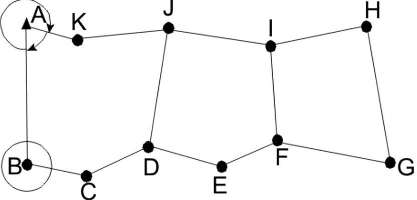
The compass rule adjustment is known as an arbitrary method of adjustment since it is possible to obtain different solutions depending on the route and observations that are used to perform the adjustment. A simple example can demonstrate this situation. Assume that a control survey is being performed, and the surveyor closes the angular horizon at each station as well as makes a few cross checks in the survey. Figure 1 depicts this survey.
Figure 1
A control traverse example.
Since the compass rule allows only one angle at each station to be used in the computations, the surveyor may simply:
- use the interior angles of the traverse to compute azimuths, using the exterior angles only as a check on the interior angles so that large measurement errors can be isolated,
- use the exterior angles to compute the azimuths of each course and use the interior angles simply as a check,
- adjust the sets of angles at each station and then use the adjusted interior or exterior angles to compute the azimuths of each course, or
- use some combination of the three previously described.
As you can see, we already have at least four different solutions to this traverse, but it doesn’t stop here.
As shown in Figure 1, there are two cross ties made between the long sides of the traverse. These cross ties could again simply be used as 5) a check, or 6) the traverse could be broken into three smaller traverses. For example, the traverse ABCDJK could be adjusted, then link traverse DEFIJ, and finally FGHI. Additionally, there are even more possible scenarios that could be used in performing the adjustment. In this manner, the surveyor is adjusting all the distances and not simply using them as a check.
The end result of all of this is that the final adjusted coordinates, distances, and directions will vary depending on the procedure followed. This is why the compass rule is known as an arbitrary method. It can and will provide different solutions depending on how the data is adjusted.
The advantage that a least squares adjustment has over an arbitrary method is that one and only one solution is possible from the work performed in Figure 1. Additionally, this solution will simultaneously adjust all distance and angle observations gathered during the survey and ensure that all geometric closures are met. There will be only one possible solution, and it will be the most probable solution for the given set of observations.
What it does not do is make bad data good. Of course, neither does any other adjustment method.
Furthermore, each observation can be weighted according to the precision of the observations. What does this mean?
By looking at Figure 1, we can see that some of the distances in the traverse are significantly shorter than others. As experience has taught, an angle observation with shorter sight distances is generally not as precise as one with longer sight distances. Thus angles such as BCD or DEF will typically have higher uncertainties and should be given more of the angular misclosure error in the traverse.
However, Table 1 shows that even with more angular correction, this does not necessarily translate into larger positional change for stations connected to these angles. For example, a 3” correction in an angle with a 100-ft sight distance will result in only a positional change of about 0.001 ft, whereas the same correction to the angle with a 1500-ft sight distance will experience a 0.022 ft change in position. It would take a 45” correction to an angle with a 100-ft sight distance to effect a similar change in the station’s coordinates.
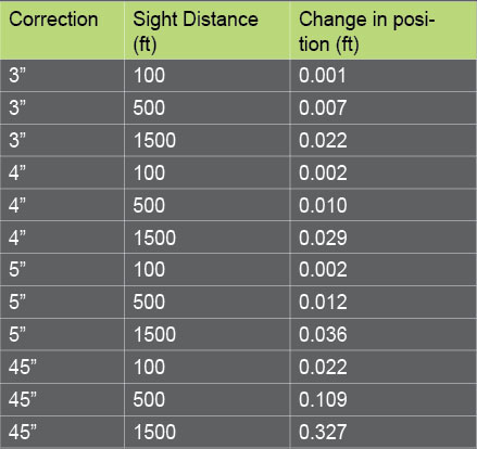
Table 1
When all angles receive the same amount of correction, which is typically done using the compass rule adjustment, this means stations with longer sight distances will experience larger shifts in coordinates from the angular corrections.
What statistics and the least squares method allow are individual weighting of observations. This is both a good and bad thing. When weights are applied properly, each angle will receive its fair share of the misclosure. However, if weights are applied improperly, the resulting adjustment will be distorted. Thus it is important to get the weighting of the observations correct.
In fact, the relative positional accuracy standards in the 2011 Minimum Standard Detail Requirements for ALTA/ACSM Land Title Surveys requires a correctly weighted least squares adjustment be performed. The proper weighting of optical observations will be covered in a later installment in this series of statistics and least squares adjustments. For now realize that when proper procedures are followed, you will obtain the most probable values for the unknowns; all observations will be used in the adjustment and be adjusted simultaneously; all geometric closures will be enforced; and as an added benefit you will receive post-adjustment statistics that will serve as an aid in isolating substandard observations.
In order to understand the least squares method, we need to understand its underlying normal distribution and statistics. In subsequent articles, I will discuss the fundamental principles of the normal distribution and the random errors that comprise it, how errors in our observations propagate through the computational process, the least squares method and its post-adjustment statistics, and how we can use these post-adjustment statistics to aid in our search for mistakes in our observations.