Two recent advances in heretofore unrelated technologies are giving birth to a new way to perform local-area metric mapping. The first is the development of small, unmanned aerial systems (sUAS), spurred on primarily by the miniaturization of autopilot components. The second is the development of novel algorithms for creating digital surface models from collections of overlapping images acquired with consumer-grade cameras in the absence of accurate exposure station information. This combination of technology makes it possible to do local-area 3D mapping with a total nonrecurring investment of under $15,000! Repeat acquisitions are enabled with a simple battery recharge.
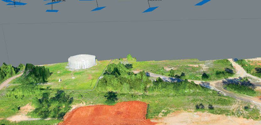
That is the good news. The bad news is that, at least with current software offerings, it is very difficult to assess the accuracy of the image mosaics and point clouds generated by these processes. Generating products from camera images requires exact knowledge of the location and attitude of the camera at the point where each image was acquired (the exposure station exterior orientation, EO). Unlike traditional photogrammetric approaches, new Structure from Motion (SfM) algorithms can solve the EO problem with no a priori location information (e.g. GPS) and no ground control points. The figure above depicts a scene synthesized from 81 images from a Canon S100 camera using no a priori camera station information.
At AirGon (a GeoCue Group subsidiary), our primary interest is in metric mapping—that is, mapping projects where we need quantitative geometric information rather than simple visualization. sUAS are useful in the space between practical ground surveys and manned aerial
missions—projects with areas up to several square kilometers. The types of projects that apply to this scenario include orthomosaics for planning, volumetric analysis, and local area Digital Terrain Model (DTM) creation. Of these applications, I think volumetric analysis will be the payday for surveyors.
SfM algorithms take a different approach from traditional photogrammetry in solving the camera location/attitude problem. The SfM algorithm generates a sparse 3D point cloud that best fits a set of match points between highly redundant (overlapping) images. This solution is what, in photogrammetry, we would call a “free net” solution. That is, it is not physically tied to the object space (e.g. ground) and hence contains scale, translation, and rotation errors. Fortunately, in a good model, these errors are uniform throughout, and thus the model can be fairly accurately tied to ground with a minimum of three ground control points.
Even better news is that the model can be scaled with the introduction of a scale bar or scale measurement. For relative computations such as volumetric analysis, no control is needed if scale is introduced into the model. This is a very big time and cost savings because GPS control is not required.
The simplest technique to use in introducing scale is to place ground targets and measure the distance between the targets, using, for example, a survey tape. An advantage of this technique is that you can always go back to measure the object space coordinates (using GPS) of the targets if absolute positioning is required. If it is not possible to signalize the mapping area, then objects of known length can be used to introduce scale.
This presents us with three levels of control for sUAS projects:
• None—This is only appropriate for visualization.
• Scale—This is appropriate when only relative (local) accuracy is needed. Volumetric analysis and length, area measurements are good examples.
• Full ground control—This is necessary when absolute location is needed. An example would be drainage analysis of an area or planning an excavation.
The question arises, of course, as to just how accurate imagery from an sUAS can be? Figure 2 is a cut-out of a control report from one of the sUAS SfM processing packages. This report tells us the residuals after fitting the model to control using a similarity transform (“projections” indicates in how many images the point occurs). This gives us a warm feeling about the goodness of our model because we see no residuals above 1.3 cm! Unfortunately, this feeling is false.
What we must actually do is withhold a number of points from the computational model and use these withheld points in an independent accuracy assessment (more on this in a future article).
Finally we have to ask the question of just how well the resultant point cloud fits the true object space. This is a very difficult question to answer without very dense ground control. Of course, if one needs very dense ground control, the entire purpose of high-speed sUAS mapping is defeated! Consider the image of Figure 3. Here we have overlaid a contour rendering of point clouds from two different SfM packages, yellow from one and green from the other. The area boxed in red shows a substantial difference between the two solutions. Which is more correct?
We think this is the most difficult question to answer. In a future article, we will explore some techniques that can be used to quantify the accuracy of the point cloud in these difficult terrain areas.
The conclusion thus far is SfM algorithms applied to imagery from sUAS can provide immediate value to surveyors for a variety of applications. The entire kit (hardware and software) can be obtained for less than $15,000. However, as in all precision work, you have to be conscious of factors that introduce error into the models and take active steps to reduce these errors. In a future article, we will explore methods of dealing with the more difficult of these such as undulating terrain in stockpiles. Until then, successful flying!