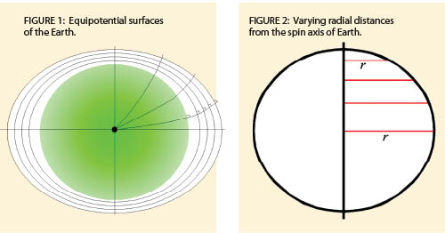
 As mentioned previously in this column, the geoid is the equipotential gravitational surface on which all elevations are referenced. An equipotential surface is where the force times distance is a constant. Gravity provides the force, and the distance is the height above this surface defined along the plumb line of an instrument. As shown in Figure 1, the plumb line is a curved line going to the mass center of the Earth.
 It is common to think of elevation as purely a distance above the geoid, but this ignores that fact that the gravitational pull of the Earth is not a constant. To understand this last statement, we must recall a little physics and look further into the effect of the spin of the Earth.
 Sir Isaac Newton defined the force of the gravity between two masses as Equation (1) where G is the universal gravitational constant, M and m are the two attractive masses, and ∆R is the distance between these masses. Because the mass of the Earth is a constant, the combined constant for GM is currently defined as 3,986,004,418×1014m3s−2 with the GRS 80 ellipsoid. In this discussion the mass of the Earth can be thought of as a point mass at the center of the Earth, and ∆R is the distance from this mass.
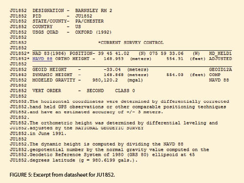
As shown in Figure 1, these surfaces converge at the poles. To understand why this occurs, we have to look at one of the motions of the Earth, which is its rotation. The rotation of the Earth causes a centrifugal force that counteracts the pull of gravity. The surface velocity caused by this spin is given by Equation (2) where v is the surface velocity, ω the angular velocity of the Earth, and r the radial distance from the spin axis, as shown in Figure 2 (opposite page).
The surface velocity will change with latitude. It is greatest at the equator and zero at the poles due to the varying radial distances from the spin axis of the Earth. Simply put, at the poles the surface velocity is zero because we are on the spin axis, and it increases as we move toward the equator where the radial distance is the greatest.
You can view this phenomenon by dipping a top in water and then spinning it. The water will fly off with the greatest velocity and distance at the widest location on the top. However, water will simply run down the top at its tip because only gravity is pulling on it. From this we see that the combined effect of these forces results in the pull of gravity being greatest at the poles and weakest at the equator.
Why Gravity Affects Measurement
A gravity model for the conterminous United States (CONUS) is shown in Figure 3. Note how the elevation of both the Appalachians and Rockies changes the gravity values. Gravity is measured in the units of cm/s2, which is defined as 1 gal where gal is named after the famous Italian astronomer/scientist Galileo.
Equipotential surfaces are defined by their ability to do work. From physics, this means that all points on any equipotential surface are determined by Equation (3). Because gravitational pull increases as we move to the poles, the distance a particular surface is from the mass center of the Earth must decrease to maintain this constant. The convergence of these surfaces has a direct impact on our leveling.
As shown in Figure 4, when we level our instrument we create a horizontal plane with our line of sight. However, if we look in either a northerly or southerly direction, the equipotential surface will diverge from our line of sight. This occurs because we are measuring only one of the two necessary components to determine orthometric heights, which are commonly referred to as elevations. We are measuring the change in distance, but not the change in gravity.
We also need to know the average gravity between the two surfaces because the distance between the surfaces changes with changes in subsurface gravity. A theoretical average gravity value can be obtained using the Prey reduction, which isEquation (4) where g- is the average gravity at a location, g is the gravity as determined at the surface, and H is the orthometric height of the location. If we combine equations (3) and (4), we obtain what is known as the equipotential surfaces geopotential number, which is given by Equation (5) where H is the orthometric height of the station and g the surface gravity at the station.
I doubt if any of us has a gravity meter to determine the surface gravity. Fortunately, all is not lost. Because the change in gravity is relatively small for a local survey, the error due to the convergence of the surfaces is less than the observational errors of our leveling, and thus is not readily discernible. However, if we level in a long north-south direction, starting at one benchmark and closing on another, part of the misclosure error in our survey is caused by the convergence of these surfaces.
Determining Leveling Height Differences between NGS Benchmarks
 How can we remove the effects of gravity without knowing gravity? Fortunately, the NGS datasheets provide us with enough information to determine the leveling height difference between any two stations. To demonstrate this, I will use an NGS benchmark station near the Pennsylvania southern border and another station near its northern border. This will demonstrate the procedure as well as the size of the error in a north-south distance of about 159 mi.
The plan is to determine the change in geopotential number C between the two benchmarks. This change is then divided by the average of the gravity values at each station. The station I selected near the southern border is JU1852, which is in Chester County, Pennsylvania. An excerpt from this datasheet is shown in Figure 5. JU1852 has a NAVD 88 elevation of 168.953 m and a modeled gravity value of 980,120.2 mgal.
From these two values and Equation (5), we can determine the geopotential number for this equipotential surface asEquation (6) where C is the geopotential number for station JU1852 in units of kgal-m, and 1,000,000 was introduced into Equation (4) to convert mgal to kgal, which simply makes the numbers look more like their orthometric heights.
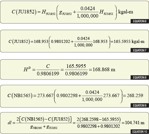 Using Equation (6), we can determine the geopotential number for station JU1852 asEquation (7). (Sorry, but the theory states that these equations must be computed in SI units. You cannot use English units in these equations.) Thus the equipotential surface passing through this station has a constant value of 165.5955 kgal-m. This is known as the geopotential number C on the equipotential surface passing through JU1852.
The problem with this value is the mix of length and gravity units. To get around this mix of units, the NGS uses a theoretical value for gravity at 45° latitude of 980.6199 gal for the GRS 80 ellipsoid. The dynamic height HD reported on the datasheet is defined asEquation (8) where the gravity value has been converted to units of kgal to match the geopotential number units of kgal. From the datasheet in Figure 5, we see that the dynamic height for this station is 168.868 m. Dynamic height is strictly theoretical. But it does have the advantage of having only length units and the fact that any two points with the same dynamic height are on the same equipotential gravitational surface.
If we perform a long north-south differential leveling line, how can we remove the effects of the convergence of the surfaces caused by varying gravity values without actually measuring them? The answer to this question lies again in the data that the NGS provides us.
As previously shown, the geopotential number of JU1852 was 165.5955 kgal-m. A point near Pennsylvania’s northern border is NB1565, which is in Tioga County, New York. The NAVD 88 height for this station is 273.667 m with a modeled surface gravity of 980,229.8 mgal. Making the appropriate substitutions into Equation (6) yields a geopotential number for the equipotential gravitational surface passing through NB1565 of Equation (9). This means that the difference in geopotential numbers is 268.2597 − 165.5955, or 102.6642 kgal-m. To get the leveling height difference, we simply need to divide this difference by the average of the two surface gravity values at the stations or Equation (10).
Notice that if we simply had used the NAVD 88 orthometric heights as reported on the datasheets, we would have computed a difference of 104.714 m. This means the difference in the equipotential surfaces at the northern and southern borders of the state is 2.7 cm or 0.09 ft. Of course, that is over a distance of about 159 mi. Yes, this difference is small, but it exists, can be computed, and can be removed so that only true leveling errors are adjusted.
Determining Leveling Height Differences between Other Stations
Unfortunately, most surveys do not run from NGS benchmark to NGS benchmark. Assuming that the orthometric heights of your benchmarks are accurate, how can you get the gravity values for these stations?
First you must have approximate geodetic positions (latitudes and longitudes) for each benchmark. This can be obtained by careful scaling off of a USGS quadrangle map sheet or with a code-based GPS unit like your cell phone. With these positions in hand, go to the NGS geodetic toolkit. This suite of software packages has one that will predict the surface gravity for any location in the United States. The actual package can be found at www.ngs.noaa.gov/cgi-bin/grav_pdx.prl. The software will provide a modeled gravity for the location you enter.
As stated previously, this error is extremely small over long north-south distances, and thus, in practice, is typically ignored. In fact, an equipotential surface that is 200 m above the geoid will converge only a little over 1 m at the poles, which is really small for the distance between the two locations.
However, now you know the rest of the story, how the National Geodetic Survey created benchmark “elevations” in the first place, the importance of gravity, and why they are currently working on the GRAV-D program, and the significance of the dynamic heights that are listed on their datasheets.
At the conclusion of the GRAV-D program we should have an accurate geoid model for the United States. This, in turn, will allow us to obtain accurate elevations from our GNSS receivers, which may eliminate the necessity of occupying a benchmark to get an accurate elevation on a project. The future is coming, and it is not too far away.