Localization Process Statistics

Note that all of the computations discussed in the previous article occur in the background on the controller. As a surveyor you will never see the temporal map projection coordinates or the transformation parameters. What you will see is the fit between the two reference frames in the form of residuals. At this point, it is up to the surveyor to decide whether the fit is adequate enough to continue. 

Here is where both experience and statistics can help. If you have done this localization properly several times you will become accustomed to the size of the residuals you can expect from your surveys. But what happens when you are using someone else’s established local coordinates for your control? At this point we must be cognizant of the typical errors from your GNSS receiver as well as from the other survey. Let’s look at an example.

Assume that you are using a GNSS receiver where the manufacturer claims an RTK survey horizontal accuracy of 10 mm + 1 ppm and a vertical accuracy of 15 mm + 1 ppm. What is the maximum size of the residuals that should be expected from a survey performed correctly? First, we must realize that the manufacturer-specified accuracies are only at 68% probability and that they do not include the setup errors of the receivers on the stations. 

These setup errors can sometimes be large. For example, if the GNSS receiver is handheld during the performance of the localization part of the survey, the receiver will wobble as the user tries to maintain a stationary position over the point. Even a small wobble by the user can result in significant errors at the typical 2-m height of the receiver. You can expect anywhere from 3 mm to 6 mm of error when the field person is being careful. However, I have seen rod persons who were more interested in their cigarette, cup of coffee, or something else than they were in the circular bubble on the rod. 

Thus, it is always wise to require a tripod support for the rod when doing the localization part of the survey. You will note that I did not state a bipod support. The reason is that the bipod leaves one side of the setup with a vertical leg, which is the rod side. Any wind from a passing vehicle or nature can catch the receiver and bring it crashing down with a bipod support. I have witnessed this several times in my years of teaching and have even been hit by one receiver when my back was turned to help another field crew member.

Calculating Error

Suppose that the receiver is supported by a tripod and that the care in setup was taken yielding a horizontal setup error, Shr, of ±1.5 mm, and a vertical error, Svr, of ±3 mm. Remember that the rod height is not a perfect 2 m and that the point of the rod sits in a depression on the monument/rebar/wooden hub/nail, otherwise known as the station. 

Using error propagation theory and assuming the distance from the base receiver to your rover, which is occupying the control point, is 5 km, the 99% combined error for the horizontal portion of your survey is shown in Equation (1) where 2.576 is the critical value from the normal distribution for 99% error. The 99% probable error for the vertical component of this baseline is shown in Equation (2).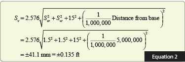 

The multiplier of 2.576 assumes that the station was observed for more than 30 epochs of data. Typically, these stations should be occupied for a minimum of three to five minutes using a 1-second epoch rate yielding anywhere from 180 to 300 observations. For example, if you were using only 10 epochs of data at each station, then the multiplier would come from the t distribution, which is 3.25 for the nine redundant observations in this case. 

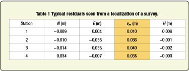
Table 1 shows the residuals from a localization where the horizontal transformation parameters were a = 0.43139, b = 0.052838, TE = 412.587 m, TN = 1866.123 m, re = −1.574″, rn = −3.205″, and Th = 0.660 m. Again, these transformation parameters are not shown to the user typically. Instead, the user will see the residuals in the columns headed by N, E, and H in Table 1 and asked whether these residuals are acceptable. 

They will not see the column headed by vne which is the combined horizontal residual component and must be computed from the horizontal residuals in the northing and easting for each line using Equation 3.

From our previous analysis of the 99% errors in the horizontal and vertical components of the line and assuming that all four control points are 5 km from the base, we see that all the vertical components are well inside Sv maximum allowable error of ±0.041 m. From the values in Table 1, we see that three of the four combined residuals, vne, are greater than the estimated 99% error of ±0.029 m. This means that there is a problem with the horizontal component of the transformation. 

It may also be noted by the signs of the residuals where 8 out of 12 are negative. Theory states that there should be as many negative as positive residuals. However, always remember that this is a sample of data, and thus small variations from theory can be expected.

How to Interpret Error

The problem for the surveyor is to decide whether to accept the localization as is, repeat the localization and try to obtain better results, or check the values of the local control station coordinates. Not knowing the purpose of this survey, its intended use, or the field procedures employed to obtain this transformation, it would be difficult to say what the most appropriate action is in this example, but this is what the owner of the data, the surveyor, is paid to do. 
However, because three of the four combined horizontal errors failed the 99% allowable error by close to the same amount, I suspect it may have to do with field procedures and a handheld rod versus a fixed rod supported by a tripod or bipod.

What is important to note in this and the previous article is that not all coordinates available in surveying are from the same reference system. When two different coordinate systems are used, the difference in these systems must be resolved. This is easily accomplished using software that the manufacturers provide with their equipment. However, the decision to accept or reject the transformations is not always as easy to determine. 

Additionally, it is important as you determine coordinates for control that you always note their reference frame for future use. This is part of the metadata for the coordinates. When handled properly, the fact that there are several different reference frames that surveyors must work in is not a problem. However, incorrectly handling a combination of different coordinate systems will typically result in a poor survey.