Estimating Uncertainties

In the previous article (January 2016), I point out the unreliability of sample standard deviations as estimates for population standard errors when the number of repeated observations is very small, which is typically the problem in surveying.

In this article I look at how we can estimate the standard errors for observations based on estimates for setup errors, leveling errors, and instrument-specific accuracies using error propagation principles. Note that this method of estimating uncertainties in observations is not new, since R. Ben Buckner, Edward Mikhail, and Gordon Gracie published these concepts in the early 1980s.

Estimating Centering Errors

When a survey is performed, the surveyor is mathematically trying to determine the coordinates of a mathematical point. In real life this point may define the center of a stone wall or a punch mark in a rebar.

Assume a tack is placed in a hub to physically represent the point on the ground. Our ability to center over the tack varies according to our individual abilities, care taken in the process of setting up the instrument, adjustment of an optical plummet and circular bubble, and width of the depression in the tack. For example, a depression on a tack is about 0.01 ft in diameter whereas a one-sixteenth-inch drill hole in a rebar is about 0.005 ft in diameter. With an optical plummet that is in adjustment, we can sight on what appears to be the center of a physical monument.

However, our ability to center precisely on the point becomes limited by the size of the point and our own physical limitations. For example, our centering errors will be larger on a 1-inch iron pipe than on a depression in a monument or a concrete nail. Of course, we are also limited by the calibration status of the levels, optical plummets, and circular bubbles on the instruments, as well as our patience in truly achieving what appears to be centered.

However, if care is taken with a well-defined point we should be able to achieve a centering error of ±0.005 ft on a tack or ±0.003 ft on the small drill hole.

Now assume that the rod is being held by a crew member who is cold or distracted, leaving the circular bubble 5 minutes out of level on a 6-ft sight height. This would yield a target that is 0.009 ft additionally from the center of the point.

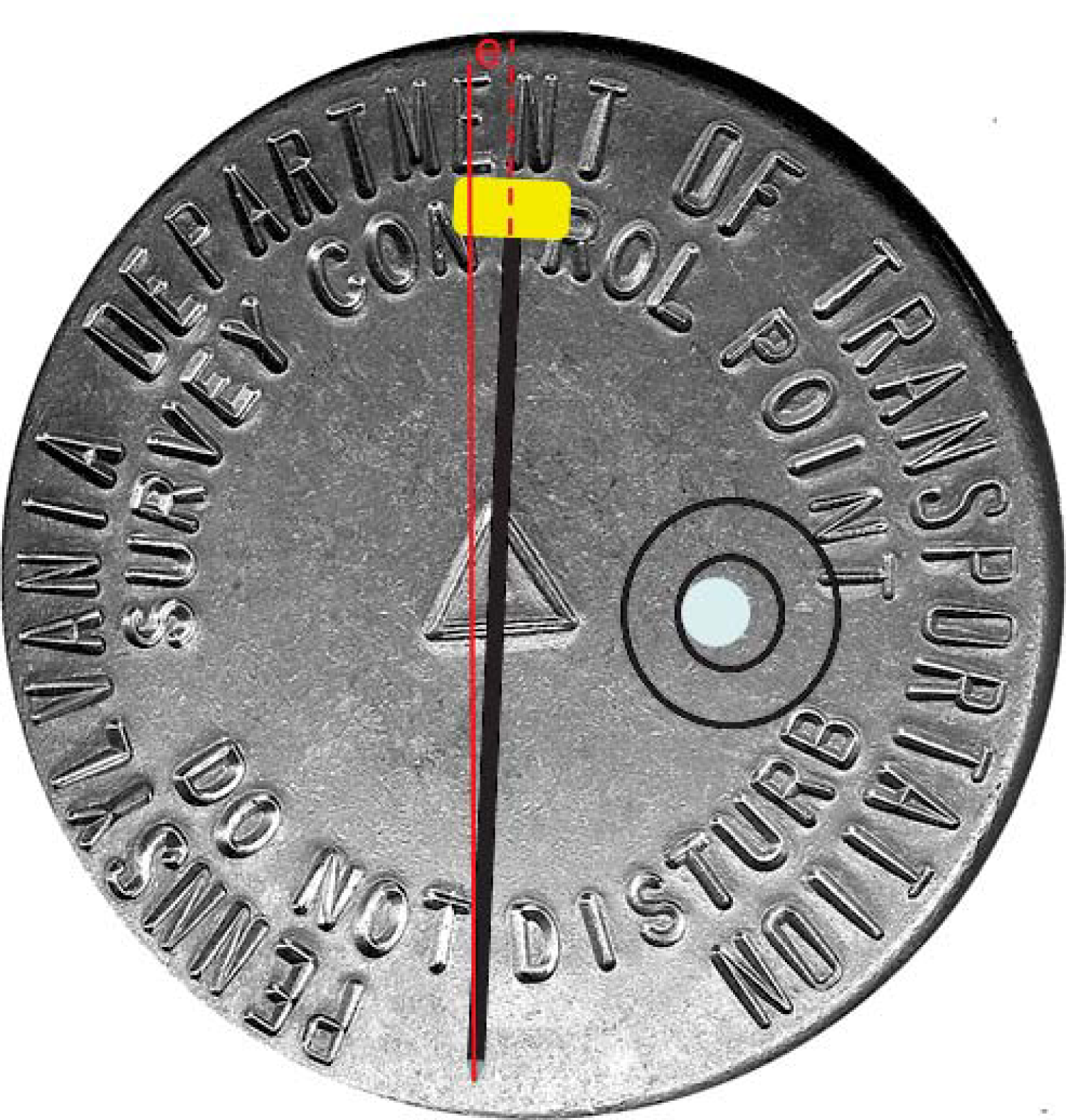
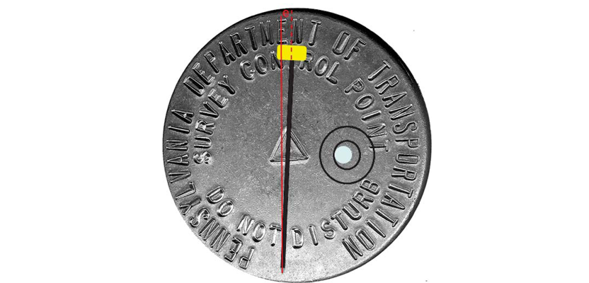
Figure 1: Sources of centering errors with a well-defined point.

There are two major sources of errors when setting on a well-defined point, which is shown in Figure 1. The first is the location of the optical plummet, plumb bob point, or rod point with respect to the center of the depression on the monument. Since a well-defined point has a depression that is typically within 2 mm in width, we can assume that a rod set in this depression will be within one-half of its width or within ±1 mm, or ±0.003 ft.

However, if an optical plummet is used, the ability of the user to center an instrument over the depression in the monument depends on his or her own physical limitations and the calibration status of the optical plummet. These errors can thus be much larger than that obtained for a rod set in the depression. For now we will assume they are the same, but this does speak to the need to check the optical plummets on your instruments often and calibrate them when they are out of adjustment.

The other major source of error is the height of the instrument or reflector above the monument. For example, a reflector rod has a 40’ circular bubble, whereas the instruments level vials are typically in the range of 20”to 30”. Assume that the bubble is off by 0.2 divisions or 8’ for the rod and 6” for the instrument.

The amount that the instrument will be off in centering is determined using the well-known formula as shown in Equation (1) where S is the centering error of the reflector/instrument over the point, R is the height of the reflector/instrument over the point, and θ is the amount of leveling error in radian units. Assuming a 5.6-ft height of the target and instrument over the point, we can compute the centering error in the target to be about ±0.013 ft for the reflector and 0.0016 ft for the instrument.

To determine the overall centering error in the instrument or target over the point we need to apply some simple error propagation where the overall error is the square root of the sum of the individual errors squared, or as seen in Equation (2).

Thus, using the numbers above, we see that the centering error for the instrument is about ±0.003 ft for the instrument and ±0.013 ft for the target, assuming we have a well-defined point and that the level vials—whether real or electronic—are in calibration. Again, this speaks to the importance of keeping your instruments in calibration.

Analyzing Errors in Distance Observations

Not all distance observations have the same uncertainty. For example, the manufacturers of EDMs tell us that the precision of repeated observations by their instruments is a constant error a (for example, 3 mm) and a scalar error b (for example, 3 ppm). The scalar portion of the precision tells us that the uncertainty of an observed distance depends on its length. The constant portion of the error tells us that the error is more significant for short distances, which results in lower distance precisions for these observations.

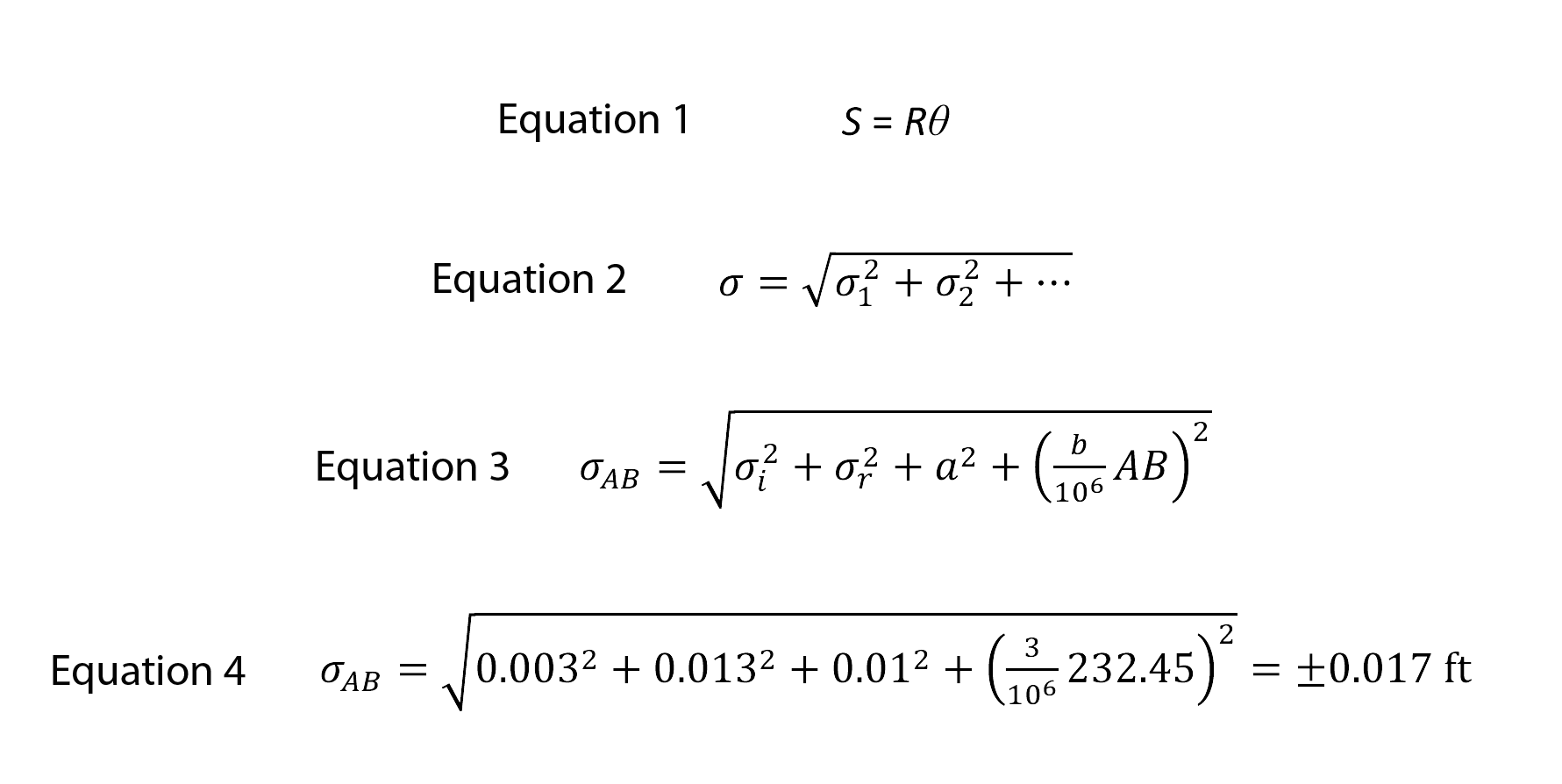However, as was stated previously the centering errors also contribute to the overall uncertainty of an observation. No matter the size of the error you estimate, these errors contribute to the overall error in the distance using Equation (2) or as shown in Equation (3) where σAB is the estimated standard error in the observed length between A and B; σi and σr are the estimated uncertainties in the setup of the instrument and reflector, respectively; and b is the scalar error in parts per million—for example, b is the 3 in 3 ppm.

Thus, if we practice due diligence in setting up the total station and reflector over a well-defined point for a distance of length 232.45 ft with an EDM having manufacturer’s specifications of 3 mm (0.01 ft) + 3 ppm, the estimated error in the observed distance is as in Equation (4).

Note that the error in each distance will be different and depends on the length of the distance and the calibration status and care in using the equipment. If care was not taken in holding the reflector over the point and we estimate the centering error to be ±0.01 ft for both the instrument and reflector, then the error in the distance would be ±0.019 ft. Note also that if the optical plummet of the instrument is off by 5 min on a 5.6-ft setup, then the setup error over a well-defined point will be ±0.008 ft.

These differences are small for each scenario, but remember that the goal is to correctly estimate the standard error for the observation so that its observational error is returned during the adjustment and not spread to other observations. Thus, the weight for the distance with an estimated standard error of ±0.013 is about 3500, whereas the weight for the distance with an estimated standard error of ±0.019 would be about 2700. Now imagine or compute the amount of error in a distance when setting over a 1-inch iron pipe, or the center of a 6-ft-wide stone wall!

In the next article in this series, I will explore the errors in angle observations. Until then, happy surveying.

References

Buckner, R.B. 1983. Surveying Measurements and Their Analysis. Landmark Enterprises, Rancho Cordova, CA.

Ghilani, C. 2010. Adjustment Computations: Spatial Data Analysis. Wiley & Sons, Inc., Hoboken, NJ.

Mikhail, E. and G. Gracie. 1981. Analysis and Adjustment of Surveying Measurements. Van Nostrand Reinhold, New York, NY.