Elementary Statistical Procedures 

In this article, I assume that a least squares adjustment has been performed. Unfortunately, many novices believe that their work is done because they now have a solution to the unknown station coordinates. However, nothing is farther from the truth. It is at this point that the real work begins in analyzing the results of the adjustment and checking the data for blunders. In this and the next article, I present statistical methods that can be used to help identify blunders in the data.

One of the easiest statistical methods used to identify potential blunders in observations is checking the acceptable range for the residuals using the t distribution. However, this method requires valid a priori (prior to the adjustment) standard errors for the observations.

I discuss how to obtain these estimates in a previous series of articles titled “Correctly Weighted Least Squares Adjustment” (See xyHt Jan., Feb., and April, 2016). If this method is used, then the critical value from the t distribution can be used to determine an acceptable range for residuals after the adjustment.

While this method can be time-consuming, it can be simplified by using the largest estimated standard error or the average estimated standard error for a particular set of observations. This is true because from experience I have noted that often the estimated standard errors for angles and distances in a survey lie in a small range. It can also be used in the field when trying to determine if a GNSS localization should be accepted.

As an example in a horizontal least squares adjustment, assume that the largest estimated standard error in an angle observation is ±4.0″ where all the estimated standard errors for the angles lie in a range of ±2.9″ to ±4.0″. Furthermore, assume the least squares adjustment had nine redundant observations or degrees of freedom. The residual for a particular angle observation is 9.8″. Typically, statistical blunder detection is performed at a confidence level of 95% to 99.9%.

Using the t distribution, a range for the residuals with this observation can be computed as shown in Equation (1).

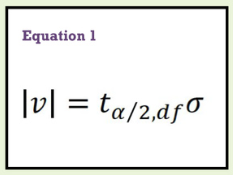In Equation (1),

• v is the residual after the adjustment,
• t /2,df the critical t value from the t distribution based on upper-tail percentage points,
• df represents the degrees of freedom or redundant observations in the adjustment, which is 9 in this example, and
• the largest estimated standard error for the angle observation.

I will first perform this test at a 95% confidence level with equal to ±4.0″ and t 0.025,9 of 2.26, with a two-tail critical value for t at a level of significance of 0.05 or (1 Ð 0.95).

Since the residual for the observation is 9.8″, we can see from Equation (1) that |9.8″| > 2.26(±4.0″) = ±9.0″. Thus, we see that the 9.8″ residual is greater than estimated at a 95% confidence level given the largest estimated standard error of ±4.0″. We may have uncovered an observational blunder, but further discussion is necessary.

Now it is time to use the actual estimated standard error for the observation, which is ±2.9″. Again using Equation (1) we find an acceptable range for the residual but this time at 0.01 level of significance, which represents 99% confidence level.

Using Equation (1) and a critical t-value of t 0.005,9 =3.25, we find the 99% range for the residual is ±9.4″=3.25(±2.9″). At the 99% level of confidence the observation’s residual of 9.8″ is outside the acceptable range. The observation should be removed from the adjustment as a blunder and reobserved.

However, it should be noted that if we had done this test at 99.9%, the critical t value would be t0.0005,9, which is 4.78, and the allowable range for the residual is ±13.9″, which equals 4.78(±2.9″). At a 99.9% level, an observation with a residual of 9.8″ would not be detected as a blunder.

Thus, it is up to the practitioner to decide how much error is too much for the type of survey being performed. Statistics can identify only what observations should be investigated as possible blunders. The surveyor must decide whether to accept the fact that he or she and colleagues are human and can commit blunders or not.

To aid in this decision, remember that a 99% confidence level means that 1 out of 100 observations, which do not contain a blunder, will be misidentified as having a blunder. Since the likelihood of a blunder being present is typically higher than this, the observation is more likely a blunder, but we can never say this for sure. In fact, since we never know the distribution of blunders, we are never positive that a blunder did occur. It simply reduces down to what are you willing to live with and what you will reobserve or remove from the adjustment.

However, from this example it is easy to see that it really depends on the accuracy of the estimated standard error in the observation and the confidence level that is chosen to perform the test. While better statistical methods are available in identifying blunders in observations, the check of the residuals is quick and easy to perform.

For example, you could use a spreadsheet to determine the appropriate critical t value and the acceptable range for the residuals at your chosen level of confidence. For the previous example at 95% confidence level, which is also called a 0.05 level of significance, simply type into Microsoft Excel “=tinv(0.05,9)” without the quotes. Excel will then determine the critical t value as 2.26, or you can type in “=tinv(0.05,9)*4.0″ to obtain the 95% confidence interval of ±9.0”.

This equation can then be quickly modified for the 99% confidence interval with a ±2.9″ estimated standard error by changing the equation to “=tinv(0.01,9)*2.9″ to obtain the range of ±9.4”. It should be noted here that Excel simply requires 0.05 or 0.01 be typed in for the confidence intervals. It always assumes that the determined critical value is for a two-sided interval.

As another example, assume we are trying to decide whether a GNSS baseline vector from a static survey contains a blunder. The manufacturer states that for a static survey, the estimated error is 3 mm + 0.5 ppm. However, if you have been reading my previous articles, you also realize that we need to consider the setup errors.

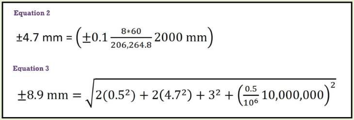
Assume that a fixed-height tripod has been used and that the level bubble on the tripod is properly adjusted. In this case, if we assume that we have the bubble within ±1 division of level at a 2.000 m height, the centering error due to misleveling is as seen in Equation (2) (Note that 206,264.8 is a conversion factor for arc-seconds to radians.)

Additionally, it is estimated that the ability to center the point into the monument’s depression is within ±0.5 mm. Since a baseline requires two setups, these miscentering errors occur at each end of the baseline. Assume a baseline that is 10,000 m long has a residual of 23 mm. The estimated error for this baseline given the manufacturer’s published estimated errors and the centering errors is as seen in Equation (3).

To perform the statistical test we must consider how many degrees of freedom there are in the observation. Statisticians state that if there are more than 30 degrees of freedom, we can use the normal distribution multipliers rather than the t distribution. Since the session was 20-min in length with observations collected every 5 sec, there were at least 240 = (2060/5) computations of the baseline.

Thus, an approximate 95% range for the residual is 1.96(±8.9) = ±17.4 mm. The residual of 23 mm is too large at 95%. However, the critical t-value at 99% is 2.576 so the 99% range for the residual is ±22.8 mm.

Thus, at 99% level of confidence, we can see that the 10-km baseline could be considered a blunder, but it is very borderline. Again, this reduces to how much error are you willing to live with.

Conclusions

While this method of blunder detection works very well, there is another method that least squares software packages can employ that makes blunder detection even easier. That is, most software uses a post-adjustment statistic known as the tau criterion. The tau criterion is a modification of a method known as data snooping, which was introduced by Willem Baarda in mid 1960s. In the next article, I explore these two post-adjustment blunder detection techniques. Until then, happy surveying.