Errors in observations can be classified as systematic or random. Systematic errors are errors that follow physical laws and can be mathematically corrected or removed by following proper field procedures with instruments. For example, the expansion or contraction of a steel tape caused by temperatures that differ from the tape’s standard temperature is a systematic error that can be mathematically corrected. Often in surveying, we correct for systematic errors using the principle of reversion. For example, we can compensate for the vertical axis of a theodolite not being perpendicular to the horizontal axis by averaging angles observed in both the face I (direct) and face II (reverse) positions. We remove the effects of earth curvature and refraction and collimation error in differential leveling by keeping our backsight and foresight distances balanced between benchmarks.
Of course mistakes (also called blunders) are a fact of life since we are human. In fact, a wise man once told me that the only people who never make a mistake are people never do anything. Mistakes are not errors but must be removed from our data. These can range from simple transcription errors to misidentifying stations, to improper field procedures. Mistakes can be avoided by following proper field procedures carefully. However there is no theory on how to remove a transcription error other than to catch them at the time of occurrence or hopefully later in a post-adjustment analysis. Actually, later in subsequent articles I will discuss methods to uncover mistakes and large random errors, which are known as outliers, in data.
Random errors are all the errors that remain after systematic errors and mistakes are removed from observations. Random errors occur because of our own human limitations, instrumental limitations, and varying environmental conditions that affect our observations. For example, our ability to accurately point on a target is dependent on the instrument, our personal eyesight, the path of our line of sight in the atmosphere, and our manual dexterity in focusing the instrument and pointing on the target. As another example, an angle observation is dependent on the ability of the instrument to read its circles in this digital age, and the ability of the operator to point on the target.
In fact, all manufacturers have technical specifications for their instrument’s that indicate the repeatability of the instrument in an observation. As an example, the International Organization for Standards (ISO) 17123-3 standard, which replaced the DIN 18723 standard, expresses the repeatability of a total station based on specific procedures in the standard. These standards were devised to help purchasers differentiate between the qualities of the instruments. They were not meant to indicate someone’s personal ability with an instrument since the pointing error is a personal error. As an example, every year I had second-year students replicate the DIN standard to determine their personal value for a particular total station. Some students would obtain values that were better than the value published for the instrument, others would get values very close to the published value, and some would get values greater than the published value. These variations were dependent on their personal differences.

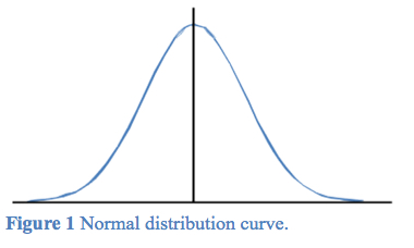
No matter whether we are using total stations, automatic or digital levels, or GNSS receivers, the random errors from observations we collect will follow the normal distribution curve. The normal distribution is based on an infinite amount of data. Thus it is not appropriate for polls performed for elected officials since the voting public is a finite number. However in surveying, we could spend our entire life measuring one distance, followed by our off-springs lives, and their off-spring’s lives, and so on forever trying to determine this single length. Of course, no one is suggesting we do this. However when we take a sample of data for an observation, the sample is from an infinite number of possible observations and follows the normal distribution and its properties. In fact, observational errors in astronomy were the reason for the creation of the normal distribution and least squares.
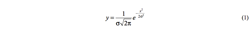
As shown in Figure 1, normally distributed data is symmetric about the center of the data. The ordinate (y coordinate) of the distribution is defined by the equation(1) where σ is the standard error of the population, and x is the size of the error.
Thus x represents the residuals for each observation with the center of the curve at zero. As can be seen in Figure 1, most errors are grouped about the center but some large random errors can and will occur. What we need to do as surveyors is find these large random errors and mistakes and remove them from the set of observations. This can happen in the field, before the adjustment, or in a post-adjustment analysis. In fact, one of the advantages of using least squares adjustment is the fact that it is possible to statistically analyze the residuals and determine when a residual is too large.
In the next article I will look at the properties of the normal distribution, what they say about random errors, and how these principles can be used to isolate large random errors and blunders in observations. I will discuss when it is appropriate to use the properties of the normal distribution. In subsequent articles, I will present alternate distributions for small samples of observations, which are typically collected in surveying. Additionally, this series of articles will look at the principles of least squares adjustments, weighting of observations, post-adjustment techniques that can be used to isolate blunders in observations, and methods to meet standards. Until then, happy surveying!