The F Distribution

Please note that the mathematical language used in this version of the article may be formatted incorrectly, due to no fault of the author. Please reference the details of Equations (1) and (2), and check with our print or full digital issue if unsure.

In previous articles on sampling statistics, I covered the t and χ2 distributions and their uses in surveying. The final sampling statistic I discuss is the F distribution, developed by R.A. Fisher and G.W. Snedecor. The F distribution is used to compare two sample variances, which are typically presented as their ratio.

In surveying we use this distribution to compare the reference variance from a minimally constrained least squares adjustment with the same statistics from a constrained least squares adjustment. We also use this statistic to compute error ellipses at a 95% level of confidence, as specified in the 2016 Minimum Standard Detail Requirements for ALTA/NSPS Land Title Survey Standards (ALTA/NSPS, 2016).

Constrained Adjustments

It is well known in surveying that in order to check geometric closures for a survey, some observations must be held fixed. For example, in a differential leveling survey, at least one station must have a “known,” which we call a controlling benchmark. In traverse computations we need to “know” the coordinates of one station to fix the traverse positionally in space and one course’s direction to fix the traverse rotationally in space. The reason for the quotes in the previous two sentences is that we can also just assume these values so that they do not have to be known in any recognized coordinate system.

However, without these observations fixed, any adjustment is impossible. When we fix the minimum number of observations in order to check geometric closures, this is known as a minimally constrained adjustment. In this adjustment, the observations need to agree only with each other to satisfy geometric closures.

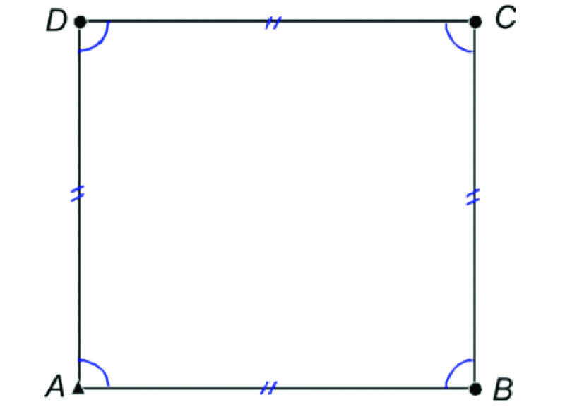
A simple four-sided traverse

Example: Assume we have a simple four-sided traverse as shown in Figure 1. If we assign coordinates (5000, 5000) to the station A and fix the azimuth of course AB to 90°, the coordinates of stations B, C, and D can be computed without requiring the angles at A and D or the length of course DA. These three additional measurements, which are called redundant observations or degrees of freedom, are used to determine the misclosure of the traverse.

For instance, the angle at A is used to compute the angular misclosure of the traverse, while the angle at station D and the length of DA are used to determine the linear misclosure of the traverse. Thus, these three unknown misclosures are determined with the three additional observations. With these additional observations, we can adjust the traverse by any means suitable.

However, if a least squares adjustment is performed, a reference variance for the adjustment is determined (as discussed in a previous article). Since this adjustment has only a minimum number of redundant observations, which are necessary to compute the misclosure of the traverse, it is said to be minimally constrained. Some academics refer to this as a free adjustment.

Now assume that we also know the coordinates of station C in the survey. This introduces more control in the form of a second set of coordinates for station C. This is an over-constrained adjustment, which can be called simply a constrained adjustment here. It is called this because the addition of coordinates for station C provides more redundant observations than are required to compute the coordinates of the traverse.

If a least squares adjustment is performed with stations A and C fixed in position and course AB fixed in direction, our observations now have to fit geometrically and match the coordinates of the two stations. This adds two additional constraints to the computations, which are the coordinates of station C.

Okay, this is a simplistic example. But how many times have you been asked to fit your survey to control created by another survey? How many times have you run into problems when this occurs? You experience these problems because your survey is now over-constrained, which isn’t a bad thing. It simply means that you have more checks on your survey data.

Example with errors. Assume that you are performing the survey using state plane coordinates, which starts at one control station with an azimuth, passes through another station with state plane coordinates much as in Figure 1, and ends back at the first station. If only one control station and azimuth are used, the traverse will close according to the precision of the observations.

Barring any blunders in the data and an appropriate weighting model for the quality of the observations, a least squares adjustment of this minimally constrained survey will result in a reference variance that should pass the goodness of fit test.

However, if the distances are not reduced properly to the mapping surface, your observations will not agree with the coordinates of the control stations. Thus, the coordinates and adjusted observations for all the other stations will be incorrect.

However, if both control station coordinates are included in the adjustment, the reference variance will be considerably bigger than the minimally constrained adjustment because the distances are not reduced to the mapping surface, and thus their corresponding residuals will be larger since they contain the difference between the observed horizontal distance and its equivalent grid distance. It is likely that the reference vari- ance in this adjustment will not pass the goodness of fit test.

A comparison of the two adjustments can be made with the F distribution, which checks to see if the ratio of the two reference variances statistically equals one, that is, if the two reference variances are equal to each other in a statistical sense.

Equation 1, Equation 2

The F test is as in Equation (1) where:

• S 21 is the larger of the two reference variances from the adjustments
• S 22 is the smaller,
• [ax] is 1 – P where P is the percentage point probability of the test, which is typically 0.95 in surveying,
• v1 is the number of redundant observations in the adjustment with S 21 for its reference variance, and
• v2 is the number of redundant observations in the adjustment with S 22 for its reference variance.

When Equation (1) is true, the adjustment is said to fail the test, and thus the ratio of the two reference variances are not equal to 1; that is, S21 ≠ S22. It should be pointed out here the S1 in Equation (1) should always be the larger of the two reference variances.

Why are they not equal? Typically, this is because the constrained adjustment (that is, the adjustment with both control station coordinates held fixed) has residuals that are much different from the minimally constrained adjustment. The reason is that the distances were never reduced to the mapping surface and thus are either longer or shorter in length than they should be. Thus, the F test is an indicator of the presence of a systematic error in the observations.

It also may not pass if the EDM/reflector constant is incor- rectly entered into a total station. For example, our second-year students check this constant each fall with their assigned equipment. One year, the students noticed a 30 mm offset and proceeded to enter it into the total station as a 30. However, a check of the instrument’s manual indicated that the manufacturer assumed that the offset is always negative and had directions to enter it as 30.

The result was an instrument that was off by 60 mm, which other students used for the entire school year. This mistake was not uncovered until the instruments were calibrated the following year. If this instrument had been involved in the survey, the F test might have uncovered the presence of this systematic error also because the residuals in the constrained adjustment would have been about 0.2 ft larger than the minimally constrained adjustment.

Error Ellipses

Another use of the critical values from the F distribution is to create 95% error ellipses. The standard error ellipse from a least squares adjustment has a probability of only 35% to 39%. This is well below the 95% mandated by the ALTA/NSPS standards (ALTA/NSPS, 2016).

The critical values from the F distribution are used to determine the multiplier necessary to create a 95% error ellipse. The multiplier for increasing the probability of the standard error ellipse depends on the number of redundant observations in the adjustment and is given by Equation (2) where v is the number of redundant observations in the adjustment, 0.05 is the percentage points determined from 1 – 0.95, and c is the multiplier used to create 95% error ellipse axes.

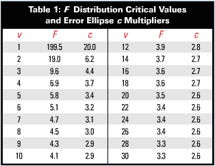
The critical values from the F distribution can be looked up in the 0.05 F distribution table or computed in the Excel spreadsheet using the function Finv(0.05,2,v) where v is the number of redundant observations in the adjustment.

Table 1 lists the multipliers for adjustments having various numbers of redundant observations, v. Note that for a simple closed traverse with three redundant observations, the multiplier is 4.4. Also note how the multiplier stabilizes with 16 or more redundant observations.

In the next article I discuss exactly what a least squares adjustment is. In a future article, I present how error ellipses are computed.

Reference

ALTA/NSPS. 2016. Minimum Standard Detail Requirements for ALTA/NSPS Land Title Surveys accessed on April 25, 2016.