The Chi-squared Distribution

In my most recent article (August 2015), I discuss Student’s t distribution and how its properties can be used to isolate blunders in observations. Another sampling distribution that is commonly used in least squares adjustments is the χ² (chi-squared) distribution. It appears in the form of what is typically called the “goodness of fit” test. To understand the value of this test, we need to understand basic concepts about the weighting of observations in a least squares adjustment (Figure 1). 

Least Squares Adjustment

Figure 1

One of many advantages that a least squares adjustment has over the compass rule or any other adjustment method is that we can apply weights to our observations, which control the size of the corrections to the observations. The manufacturers of electronic instruments such as the EDMs and digital theodolites state the precisions of their instruments in terms of accuracy standards. For example, you may own a total station with an ISO 17123-3 standard for angles of 3″ and distance accuracy of 3 mm + 3 ppm. However, this is only part of what determines the final accuracy of your angles and distances.

Other things that control the accuracy of your observations are the abilities of the user to point on the target and set the instrument and target over a point, the calibration status of the levels and optical or laser plummets, the number of repetitions of the observations, and so forth. (In the next article, I will discuss how all of these elements combine to allow you to estimate the accuracy of each observation.) We also know that longer sight distances will result in more accurate observations if everything else is the same.

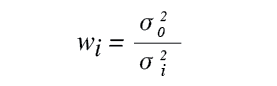
Equation 1

Least squares adjustments allow the user to individually weight observations according to the estimated uncertainty of each observation. Thus, an angle with a higher estimated uncertainty will receive more of the angular misclosure error than one with a lower estimated uncertainty. This is not the case with the compass rule adjustment, since we typically distribute the misclosure error in angles equally to all angle observations no matter how the angle was observed.

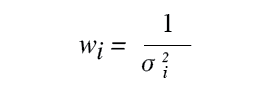
Equation 2

Weights of observations are determined as in Equation (1) where w_i is the weight of the observation, σ₁ the estimated standard deviation of the observation, and σ₀a scaling factor, which is typically assigned a value of 1. Thus, weights of observations are usually determined as in Equation (2) where σ₂₀    was assigned a value of one and is known as the a priori standard deviation of unit weight.

Determining the a Posteriori Standard Deviation of Unit Weight

After a least squares adjustment, residuals are determined for each observation. These residuals represent the errors in the observations that must be created to satisfy geometric constraints of the survey. They are combined with the weights assigned to the observations before the adjustment to determine the a posteriori standard deviation of unit weight,S₀.

Equation 3

In Equation (3), S₂₀   is the adjustment’s reference variance,w_ithe weight of each observation, v_i the residual for each observation,  ∑wi vi2 the sum of the product of the weights of each observation times its residual squared, and redundancies the number of redundant observations in the system.

Note that the number of redundant observations is also sometimes referred to as the degrees of freedom of the adjustment. For example, if a distance observation has a weight, w, of 1000 and a residual,v, of 0.02 ft, then its contribution to the reference variance is related to 1000(0.02)² or 0.4.

The key here is not how these values are computed but rather the fact that at the end of the adjustment the computed reference variance should statistically match the a priori assigned value of 1, statistically speaking  σ_{20    =}  S₂₀   .  If this is not the case, there are two possible causes.

First, there could be one or more observations in the adjustment that contain blunders. In this case, their residuals will be larger than expected. Technically speaking this means that the estimated standard deviation, σ_i, is too small for the observation.

For example, let’s assume that a distance observation has an error of 1 ft but is assigned a standard deviation, S_i, of ±0.02 ft. The standard deviation is too small for the quality of the observation, and thus it results in a contribution to the reference variance that is too large. Under these conditions, the contribution of this single observation to the reference variance shown in Equation (3) is 1/0.02²  1², which equals 2500. If this observation was given a standard deviation, σ₁ ,of ±1 then its contribution to the reference variance would be only 1/1²  1², which is 1.

The second reason for  σ₂₀    not being statistically equal to  S₂₀    is that the weights for an observation or an entire set of observations is incorrect where the accuracies of the observations are over or under what is estimated.

Goodness-of-Fit Test

The statistical method for checking whether σ_{20    =}  S₂₀     is known as the goodness-of-fit test that uses theχ² distribution. Theχ² distribution allows you to check a sample variance against a population variance.

In this case the sample variance is the reference varianceS₂₀    determined from the least squares adjustment. The population variance  σ₂₀     is the scalar used to determine the weights of the observations, which is typically assigned a value of 1. Again, if the test fails it means one of two things may have occurred, or in some cases both. The first possibility is the presence of blunders in the observations, which caused large residuals, and the second is that the observations were weighted incorrectly.

The goodness-of-fit test can be thought of as a warning flag when the adjustment fails to pass the test. It means that something is incorrect in the adjustment, but it does not tell you what it is specifically. It is at this point that the surveyor must first look at the residuals to see if any are greater thant_α/2,vS, where tis the critical value from thetdistribution with anα level of significance andvthe number of redundant observations in the adjustment.

My previous article discusses thetdistribution and its use to identify blunders in a set of data. If there are no identifiable blunders, then the surveyor should perform a cursory comparison of the assigned standard deviations for the observations against their residuals.

For example, assume that the standard deviations for the angles in the adjustment are somewhere between 2” and 3”, but the absolute value of the angular residuals are between 4” and 6”. In this case the observations are over-weighted; that is, the standard deviations of the observations used to compute the weights in Equation (2) were too low, resulting in too high a weight. When these higher weights were multiplied by their respective observational residuals, it results in a reference variance from Equation (3) that is too large.

Alternatively, it is also possible to under-weight the observations. This is the opposite scenario. That is, the standard deviations for the observations are too high when compared to their residuals. The resulting reference variance will be less than one and can be too low. In this case the standard deviations of the observations must be lowered to achieve a correctly weighted least squares adjustment.

The above scenario happens typically when the standard deviations from the observational procedures are used. Since the computed sample standard deviations for angles and distances come from observations that are not truly independent, these computed values are often misleading and lower typically than what is warranted with the instrument and field procedures.

If this all seems overwhelming, then consider the fact that the 95% error ellipses determined for an ALTA/ACSM survey must be determined from a “correctly weighted least squares adjustment,” and thus its understanding is essential if one is to perform an ALTA/ACSM survey.

In the next article I discuss the theory behind the equations that allows one to correctly estimate an observation’s standard deviation and thus simplify the process of correctly weighting a least squares adjustment. Recognize that, if the adjustment is correctly weighted, the errors in the data will return to the observations that created these errors in the first place. The result is better coordinates and adjusted observations from your survey.

Until the next article, happy surveying.