The t Distribution, Part 1

In my previous article I discuss the normal distribution and how its properties can be used to isolate blunders in observations. Recall that the normal distribution is based on an infinite number of observations.

However, in practice we never collect a population of data but rather a small sample from the population. If this sample has a large number of observations, it is likely that the mean and standard deviation computed from this sample will closely match their population values. If the sample is small then the sample mean and standard deviation may not agree with their population values.

Table 1

For example, suppose the population has 20 values as depicted in Table 1. Now, further suppose that we observe only four values from this population as shown in Table 2.

Notice how the mean, y̅, and variance, S², vary from sample to sample and further how no sample has the population mean of 22.79 or its variance of 21.29. Note that the variance is simply the square of the standard deviation.

In the early 1900s, statisticians recognized this discrepancy between a population and the samples of observations from the population, and they started to develop sampling distributions. In fact, the reason that the t distribution is sometimes referred to as Student’s t distribution is due to its origin.

(The owner of Guinness beer hired statisticians to analyze taste-test results in order to determine the most preferred recipe for his beer. From this analysis one of his employees developed the t distribution. The statistician wanted to publish his results to the world, but the owner of Guinness did not want to let other beer manufacturers know that he was using statisticians so he made the person publish the results under the pseudonym of Student. The statistician’s name was William Sealy Gosset. He published the distribution in 1908. This explains why the distribution is sometimes called Student’s t distribution.)

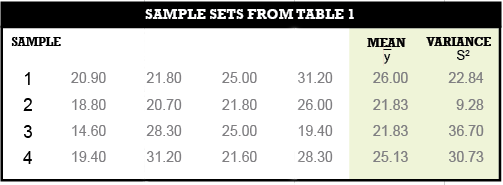
Table 2

Sampling distributions allow someone to create a range in which the population mean or variance will reside at a specific percentage of the time. They also let you test for blunders and outliers in sample sets of data. These ranges are based on the size of the samples, the sample means, and variances.

Because in surveying we typically collect a small sample of observations, we should really be using the critical values (i.e. multipliers) from the sampling distributions to create ranges for allowable errors and not those from the normal distribution.

The critical values are the multipliers we use to determine, for example, 95% confidence intervals on a set of data. A specific example of this is the ALTA/ACSM standards for the allowable relative positioning errors is a 95% error ellipse. The exception to this statement are GNSS surveys where the samples are greater than 30 observations in all but kinematic surveys typically.

Statisticians have stated that the normal distribution critical values are acceptable for developing confidence intervals when the number of redundant observations is greater than 30.

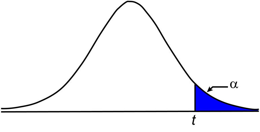
Figure 1

The sampling distributions are derived from normally distributed data. They are based on the size of the sample and the level of confidence desired. For example, the t distribution allows someone to determine a range for the population mean or sample of data. Its critical value, that is the value for t on the x axis from the t distribution, is tabulated at various levels of confidence and degrees of freedom.

It is important to note that the critical values are tabulated from infinity down to α percentage points and that it is not centered about the mean. Thus, if we want to create a 95% confidence interval, this means that we are checking with 0.05 (1 – 0.95) percentage points or what is known as a 0.05 level of significance.

As shown in Figure 1, we use 0.05 percentage points because the tabular values are determined starting at positive infinity and going back to the selected percentage of data. Since the t distribution is symmetric, which is also true for the normal distribution, the lower-tail values at a specific level of confidence are the opposite in sign of their upper-tail values.

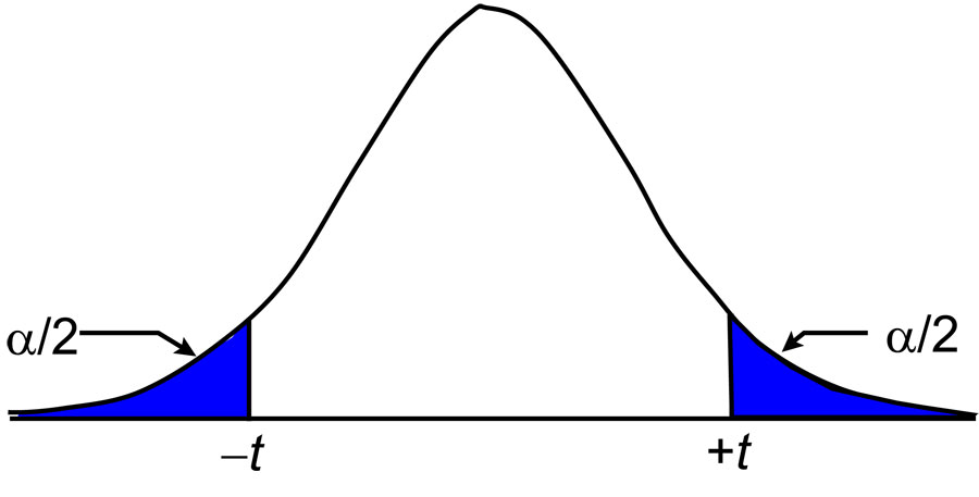
Figure 2

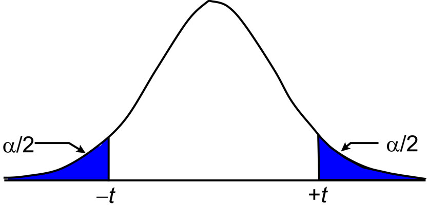
As shown in Figure 2, we can create a specific confidence interval by dividing the level of significance by 2. For example, to create a 95% confidence interval, we would need to determine the critical value for 0.025 with the appropriate degrees of freedom.

This would mean that 2.5% of the distribution is on the negative end of the graph and another 2.5% is on the positive end, leaving 95% of the data between these two values. Because of symmetry this range occurs from –t to +t.

The other sampling distributions of importance in surveying are the χ² (chi-squared), F (Fisher), τ (tau)distributions. In later articles, I discuss how each of these sampling distributions can be used to analyze surveying data. Until then, happy surveying.