By K. Olaf Niemann
The Hyperspectral-Lidar Research Group at the University of Victoria uses multisensor airborne remote sensing for vegetation mapping.
Advances in sensor technology have, in recent years, allowed the remote sensing community the luxury of simultaneously acquiring data from complementary acquisition systems. We now have the ability to characterize a surface in terms of measuring both form and function. This has been the holy grail of those who study earth surface processes for as long as we have had the opportunity to view natural landscapes from airborne and satellite platforms. Two technologies in particular have caught the attention of remote sensing academics and professionals: hyperspectral imaging, particularly in the form of imaging spectroscopy (IS), and lidar.
The evolution of passive optical imaging has evolved from multispectral scanning (MSS), where we acquire a relatively small number (typically less than 20) broad discrete spectral bands, to IS where we characterize the electromagnetic spectrum as a single continuous measurement, represented by many hundreds of spectrally contiguous measurements. Functionally, the difference between these two technologies is profound, where with MSS data we detect the presence or absence of a feature, while with IS we finally have the capability of measuring a surface process. Lidar data have been readily available for earth observation for over a decade. The nature of these data makes them ideal for the definition of surface form. Our ability to isolate ground measurements has yielded elevation models (DEM) with unprecedented levels of detail and accuracy, to the point where it has forced the more traditional photogrammetry community to rethink its approach to mapping. The added advantage with lidar data is that, along with the ground data, we also have the opportunity to address the vegetative structure through the use of the vegetation hits. These data have provided researchers with a wealth of material over the past five years to explore the vertical and horizontal structure of vegetation assemblages. Together, these two technologies provide us with a rare opportunity to examine the form and functioning of the earth surface. This article explores the workflow and specific application of a lidar/IS production and application.
 Data Characteristics
The Hyperspectral-Lidar Research Group has, since 2006, developed a toolbox that is designed to optimize the spatial integration of the multiple data sets and to use these data in the extraction of meaningful information.
An outline of the process is presented in Figure 1. The software tools were originally developed in IDL, but given the data volumes and current processing demands we have ported to C/C++ and Python and have done implementation on Linux/OSX workstations. The data collected from the multisensor airborne platform (MAP) are summarized in Table 1. Lidar’s current state of the art is well in excess of one point per square meter. The issue with the lidar data is not necessarily the posting density, as over a certain point points become redundant, but rather the power associated with each posting. It has been our experience, especially when working in forested environments, that high-density/low-energy shots will not have sufficient energy to penetrate to the forest floor and return to the sensor. These systems will typically favor the upper canopies and underrepresent the structures that are below the co-dominant canopy layers and ground. We are currently using two IS systems, designed and manufactured by Specim in Finland. The Specim V-SWIR (visible to short wave infrared) dual system consists of two separate cameras, flown on a fixed-wing platform, that are configured to image a single image cube (IS data are typically stored as a three-dimensional cube where the x and y axis represent the spatial domain and the z axis yields the spectra domain). This system yields 492 contiguously sampled spectral bands at a ground sampling distance (GSD), analogous to spatial resolution, of two meters (at 1500 m. AGL.). 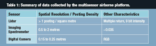 The second system is a smaller VNIR (visible, near infrared), Specim’s Eaglet spectrometer, with a spectral range of 400 to 900 nm. This system was originally intended for use with a helicopter platform that yields ca 0.5 to 1 meter GSD but is also flown on the fixed-wing to yield a 1 meter GSD.
Workflow
The workflow in Figure 1 was based on an operational need to address specific questions with the data pertaining to forest inventory and operations. The IS data are radiometrically corrected using sensor calibration data. The atmospheric correction and reflectance conversion is accomplished using a Radiative Transfer Model (RTM), in our case MODTRAN. The RTM models the transmissivity of the atmosphere, taking into account the constituent make-up of ideal atmospheres.
The result is an apparent, or at sensor, reflectance that has most of the atmospheric noise removed. To develop an exact representation of the atmospheric influences, we need to collect ground reflectance targets and apply an empirical line calibration. The most challenging initial task in processing data from the airborne system was how to integrate the two datasets spatially so that the user could be certain that the IS was pointed at the same spot on the ground as represented by the lidar data. This is accomplished in two steps. The first is through the integration of the inertial navigation data (roll, pitch, yaw, and time stamp) in the initial spatial calibration step. The second step is through the orthorectification of the hyperspectral data rather than a traditional ground-based “bare earth” orthorectificating process. We created a digital surface model for this process, gridded to the intended spatial resolution of the IS data. We sorted all of the first return heights with each of the grid cells and calculated the height quantiles. We chose the 85th percentile height as representing the top of the co-dominant canopy. The use of this height rather than the highest point smoothed the surface, removing any outliers. The IS data were orthorectified to this surface model, yielding a co-registration of the lidar and IS to within one pixel. We commonly work in two modes with these data: grid- or object-based. The grid-based mode is where we degrade the area of interest to a coarser resolution and upscale the lidar and IS data in a logical fashion. Upscaling the IS data does not involve averaging, as this would compromise the spectra. Instead, we use the lidar-based gridded data as a mask to create a series of IS layers that are analyzed separately. The object-based analysis depends on our defining morphologically based objects through a user-specified logic. For example, individual tree crowns are commonly defined using a series of morphologically based stopping rules. The result is a set of vectorized crown-objectives that serve as a basis for sampling of the IS data for further analysis.
Wetlands Mapping
One application area that lends itself to the data and analytical processes outlined here is related to wetlands mapping. This is a topical area that is of broad interest with respect to wildlife biology, landscape ecology, hydrology, and climate change.
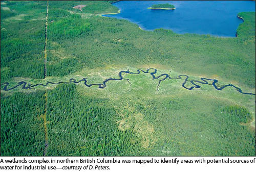
Wetlands can be defined hydrologically and biologically. They occur along a gradient from upland terrestrial through to open water. They are complex landscape elements that are commonly defined by shape. This shape and position within the landscape typically define the structure of the biological community. As earth scientists, we have had great challenges in defining and delineating the extent of wetlands, and as remote sensing specialists this challenge has become acute. The most compelling challenge to remote sensors has been to develop a method of directly measuring form, both with respect to landscape as well as vegetation stand (in its broadest sense) structure. The data that is captured by the MAP system allows us to address the form issue as well as function, at least with respect to species. To illustrate the potential for detailed discrimination of wetlands, consider an example from a project in northern British Columbia. A block of 300 square kilometers within the Horn River Basin, north of Fort Nelson, British Columbia, was flown in September 2009. The project was flown for the British Columbia Oil and Gas Commission, a regulatory organization intended to monitor oil and gas activities in the province. The purpose of the project was to develop a proof of concept demonstrating the utility of the multisensor data system and to provide data access to any interested potential user. The goal of this particular portion of the project was to map wetlands and identify areas with potential sources of water (surface and near-surface) for industrial use. Data collected is summarized in Table 2. The data processing flow outlined here was followed to prepare the entire data set for analysis. The final deliverables were submitted in late 2010. The initial processing task was to address landscape physical shape as defined by a lidar-derived DEM. Simple derivative (gradient, aspect, curvatures) models and more complex (soil wetness index) models were created. The latter is a model based on the determination of the upslope drainage area, normalized by the slope gradient. These models were initially derived at the native (2 meter) resolution and upscaled to 20 meters through the use of descriptive statistics. We upscaled these data so as to view them in more appropriate scales. The wetness (mean and standard deviation) metrics were clustered to yield five classes representing relative wetness. Next, the terrain normalized vegetation data were also subjected to a set of “biometrics” extraction algorithms to address both horizontal and vertical canopy structure (gap fraction, surface roughness, co-dominant canopy height, quantile-based moments-L-mean, L-cov, L-skew, L-kurtosis). These metrics were also clustered. Combined terrain- and canopy-based metrics yielded descriptions that corresponded to functional traits (Figure 2). When comparing the canopy structure to the derived drainage class, we can see that there is an expected relationship. The mean height of the canopy decreases with a decrease in relative drainage. In addition, the gap fraction of the grid cells also increases with decreased drainage. Finally, the skewness (or the relative loading or concentration of the vegetation point cloud: -1 to +1, where -1 is a top-loaded point cloud) increases with a decrease in drainage. The narrative from these relationships is that we can see from a single dataset that the vegetation height decreases and the spacing increases as the soils become wetter and less productive. This corresponds to known relationships in boreal wetlands where the site productivity decreases with increasing water content. A more complete understanding of the wetlands landscape is provided by the inclusion of the IS data. We used these data to yield a systematic assessment of the species structure of the landscape. For this we integrated the lidar data in the form of specific height masks. The first of these is portrayed in Figure 3. The goal of this mask was to address the top of the canopy to give us an understanding of the treed canopy. We chose to use only the reflectance from the top of the canopy to maximize the signal-noise ratio, thereby optimizing the classification accuracy. Two additional, albeit simpler, masks were also derived. These were a 0-2 meter layer to capture the shrub, and a 0 meter mask to provide an opportunity to classify lichens and bryophytes, as well as open soil and water. The final classification was carried out in three stages and compiled into a single image. A nonparametric spectral angle mapper was used as the classifier of choice given the large number of input bands. A sample of the classification of the two-meter data set is presented in Figure 4. Noted are the areas of the image that are not classified (black in the image). These areas fall between the top of the canopy and the two-meter mark. The final step was to upscale to the landscape level. To address the patterns at a regional rather than a local level, we upscaled the data to 20 meters by superimposing a 20-meter grid onto the classified two-meter dataset. There are strategies that can be adopted to resample to the coarser resolution image, but the one that we adopted used the mode (most frequent occurrence) of the class within the coarser grid cell. The result is illustrated in Figure 5. What is particularly interesting is that, while most of the area is covered by open black spruce forest (indicative of boreal wetlands canopies), there is a network of connected linear features covered by grasses. These represent the remnants of a pre-glacial landscape (pre-glacial because there are better drained features, most likely morainal or lacustrine shorelines, with white spruce and pine stands that extend across them). These features connect the smaller lakes that are scattered throughout the region. The acquisition and use of multiple complementary datasets has provided us with powerful analytical and survey tools. However, there is a cost to using these tools beyond the purchase price. It has been our experience that considerable capital has to be expended in developing spatial radiometric/atmospheric calibration techniques. In addition, the analytical toolset that optimizes mutual information extraction from these two datasets have not been widely developed, so any potential users will be exposed to a significant learning curve. Having said that though, the potential benefits from having access to both lidar and IS data for work related to the earth’s surface form and processes outweighs any initial efforts.