Editor’s note: Public awareness of the potential for interference and jamming has rightfully increased over the past few years; due partially to at least one high profile incident each of “trucker jammers,” news of battlefield jamming, the jamming event along the North Korean border, and an inadvertent interference instance of naval origin in San Diego. These are all underscored by the (past) broadband vs. GPS controversies.
While outside of battlefields the hazards have thankfully been more “potential” than “prevalent”; such hazards though could have impacts ranging from inconvenient to devastating (especially for safety-of-life applications where eLoran, ADS-B, etc are being further developed and implemented to provide much needed backup).
When it comes to high-precision positioning, solutions for rejection and mitigation of interference (inadvertent or deliberate) are not as simple as we might have been led to believe during the height of the broadband vs. GPS media flurry – the idea of tiny “50 cent” filters solving everything has been universally dis-missed. When it comes to protecting high precision GNSS against such hazards, size does matter.
We’ve been examining these issues (See the Oct 2012 and March 2013 issues in the Professional Surveyor Archive online) and are honored to present further examination in the form of an educational paper graciously provided by Dmitry Tatarnikov and his fellow GNSS engineering colleagues.
Introduction: GNSS Signals and Sources of Interference and Jamming
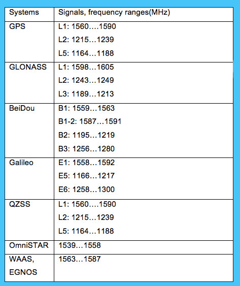
Table 1 – GNSS signals and frequencies
Currently, the Global Navigational Satellite System (GNSS) includes GPS (United States), GLONASS (Russia), BeiDou (China), Galileo (European Community), IRNSS (India), and QZSS (Japan). In addition, other satellite systems like OmniSTAR provide differential corrections. GNSS satellites transmit a variety of signals. Each signal occupies a certain range of radio frequencies. Signal power distribution over frequencies is referred to as “power spectrum.” GNSS signals and their frequency ranges are listed in Table 1.
The general goal of these signals is to be received and processed by most users to provide positioning. From the standpoint of antenna and radiofrequency (RF) circuitry of the system, it is practical to combine all the GNSS signals into two sub-bands: a Lower Frequency sub-band and an Upper Frequency sub-band. These sub-bands are shown schematically as blue in Figure 1.
A user’s positioning system can be adversely affected by interference and jamming signals of different origins. When the interference source/jamming power is of a large magnitude, the user’s system may be unable to provide a position. Antenna and RF circuits of the user’s system are potentially capable of differentiating GNSS signals and interference/jamming by frequencies. The user’s system is designed to pass the GNSS signals with the most minimum distortion possible; a frequency range of desirable signals forms a system pass-band. Contrasting, it is desirable that all signals outside the pass-band are suppressed (rejected) by the system. The frequency range outside the pass-band forms what is known as a stop-band.
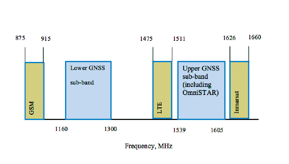
Figure 1 – Spectra of GNSS and communication systems (schematically) can be grouped into two bands: a Lower Frequency sub-band and an Upper Frequency sub-band.
Ideally, the user’s system would pass the signals within the pass-band with no distortion and would completely reject all the signals within the stop-band. Thus, frequency response of an ideal system should be as shown in Figure 2 by the thick dashed line. The zero dB indicates a case free of distortion in terms of magnitude, and minus infinity dB indicates a complete rejection. Unfortunately, such a step-like response cannot be realized. A typical practical response is illustrated in the same figure by
curves 1 and 2. This response is generally smooth; the signals of the stop-band based on frequencies close to the pass-band may possibly not be suppressed to a desirable degree. These signals are potentially the most damaging in regard to securing a quality measurement.
Thus, the largest potential sources of interference and jamming are systems operating at frequencies close to GNSS bands (e.g., high speed communication and data transmission systems). Selected examples are listed in Table 2.
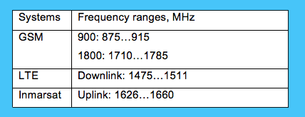
Table 2 – Signals and frequencies of communication and data transmission systems
Signal spectra of these interference/jamming signals are shown in Figure 1 (in gray). In particular, it is worthwhile to note Inmarsat and LTE transmissions are in the close proximity of the Upper GNSS sub-band. Radiofrequency components responsible for passing the signals of the desired band and suppressing the signals of the undesired band are known as filters. They are discussed in more detail in the following Section.
Radiofrequency Filters – a General Overview
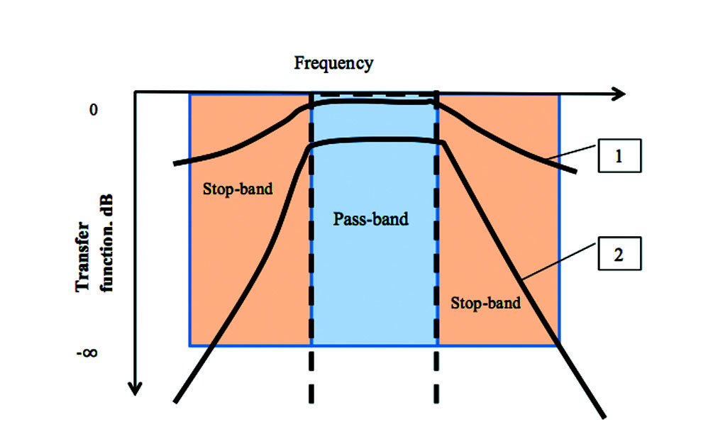
Figure 2 – Frequency response of ideal and practically realizable filters
A filter is a component that passes the signals of the pass-band and suppresses (rejects) the signals of a stop-band. Potentially, radiofrequency filters could be designed and made using
various techniques. It should be noted that an unavoidable property of a real world body [object] is to absorb some portion of electromagnetic power passing through it. As a result, the frequency response of a filter within the pass-band would never strictly equal 0 dB, which would be the case if there were no absorption. Instead, the frequency response curve is always shifted downward within the pass-band indicating that a certain loss of signal power occurs. An important practical rule derived in the filters theory (references 1 & 2 below) emphasizes the following: regardless of the technology employed in the filter construction, if the filter size is fixed then the increase (improvement) of suppression of the signals in the stop-band generally can only be achieved at the expense of increasing loss of signal power in the pass-band. In other words, for the filters of fixed size, the frequency response curves may look like those shown in Figure 2. The Filter 2 has a better slope of the suppression curve in the stop-band associated with larger signal loss in the pass-band compared to the Filter 1. An important note is with the filters downsizing, signal power loss in the pass-band increases.
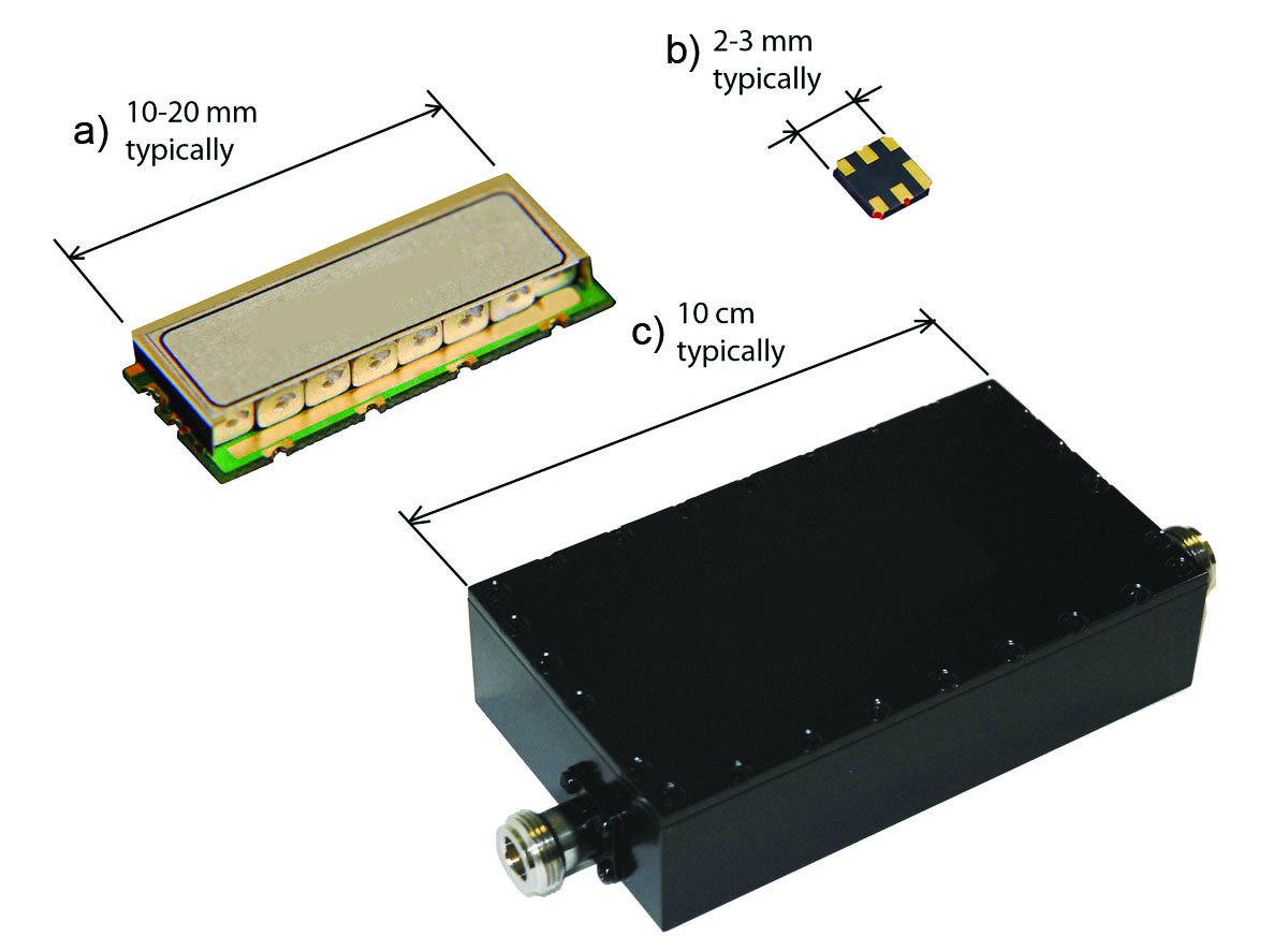
Figure 3 – Filters typically used with receiving GNSS systems. Ceramic (a), SAW (b), and cavity (c)
Some of the filters most commonly used to date for receiving GNSS equipment are of ceramic (1) and Surface Acoustic Waves (SAW) (2) types. A general view of these types of filters is shown in Figure 3 (a & b) respectively.
Typical frequency response of these filters with respect to the Upper GNSS band is shown in Figure 4 by curves 1 & 2. One may note the SAW filter, being of much smaller size, has much better suppression of signals in the stop-band compared to a ceramic one as well as a much larger signal power loss in the pass-band in accordance with statements above.
Loss of useful signal power is highly undesirable for the user GNSS systems. In accordance to the fundamental Naiquist theorem (reference 3) power loss is associated with the generation of extra noise. A loss of signal power and generation of noise results in degradation of the signal-to-noise ratio (SNR) of a user system. This, in turn, leads to signal tracking difficulties.
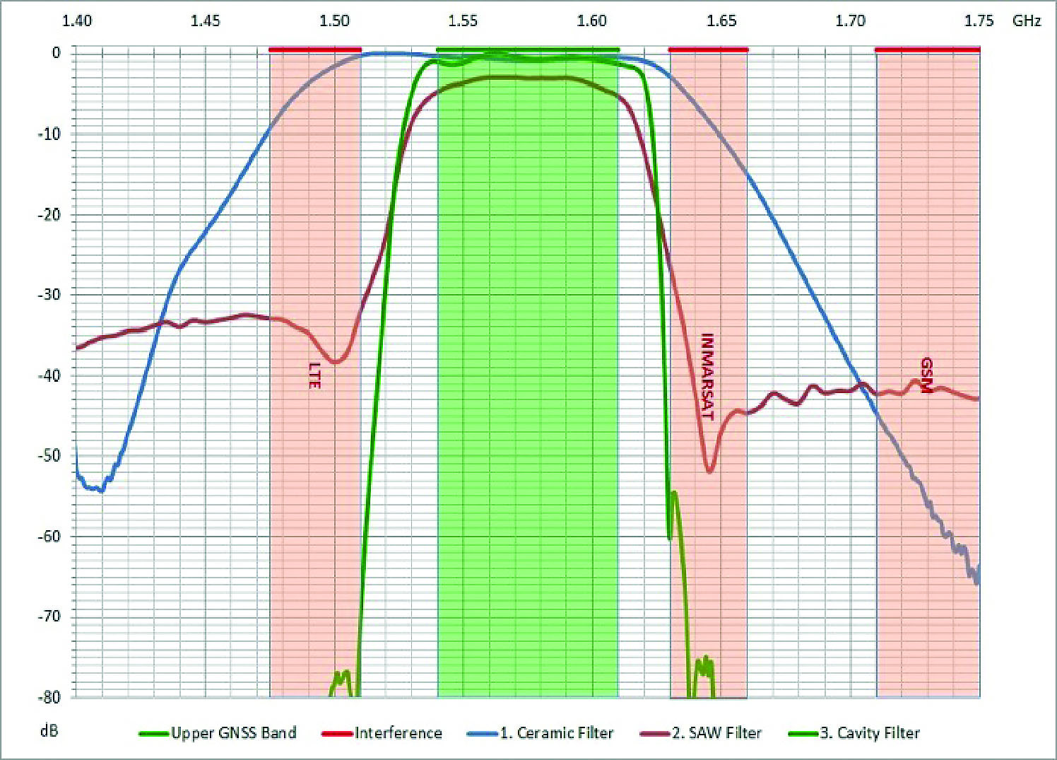
Figure 4 – Frequency response of ceramic (1), SAW (2) and cavity (3) filters (typical).
The first section of the RF portion of the receiver has a special designation – Low-Noise Amplifier (LNA). The LNA sets up the noise figure of the receiving system. For the best achievable SNR, the LNA normally is incorporated into the same housing with the receiving antenna; such an antenna is sometimes referred to as an “active” antenna. The LNA is designed to have a large gain and the smallest noise figure possible. One may check with antenna and RF circuitry foundations, and in particular with the Friis’ formulae (reference 3), to find out that no SNR degradation normally occurs after the LNA.
Therefore, it is first the LNA that is to be affected by a strong jamming. Such a strong jamming may result in the LNA being overloaded and malfunctioning. At the same time, the LNA is designed to suppress the jamming signals to protect the rest of the circuitry and to keep the highest SNR possible. Achieving these goals normally would require a combination of ceramic and SAW filters to be used. A typical block diagram of LNA is shown in Figure 5.
Referring to Figure 5, F1 is a ceramic filter, A1 is the first amplifier, F2 is a SAW filter and A2 is the second amplifier. Intuitively, and by employing Friis’ formulae, it is important to assure the gain of the first amplifier A1 is large enough resulting in the noise figure of the system is set up by the ceramic filter and this first amplifier. Large loss of useful signal associated with the SAW filter contributes to the overall noise figure growth. It should be noted with large gain of A1 given, this contribution is less significant. At the same time the jamming suppression is defined by the frequency response of the SAW filter. However, for this schematic, the amplifier A1 generally remains open to jamming due to modest filtering properties of the ceramic filter.
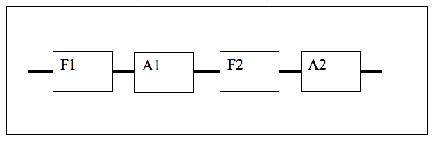
Figure 5 – Block diagram of LNA with a combination of filters
With the current technology, the best and most complete solution is provided by filters of another kind – cavity filters. A cavity filter is a chain of resonating cavities machined inside a metal body. These filters are of much larger size compared to ceramic and SAW filters. A general view of a cavity filter is shown in Fig.3c). Performance features of the cavity filters remain unattainable by other technologies. Frequency response of a typical cavity filter is shown by curve 3 in Figure 4. As seen, the cavity filter provides the same (or even less) loss of signal power in the pass-band compared to a ceramic one. At the same time, suppression of the signals in the pass-band is maximized and unprecedented. In particular, Inmarsat and LTE transmissions are suppressed by a cavity filter by the amount of 60 dB, with the smallest which is 6 orders in terms of power. Demonstrated in the block diagram of Figure 5, the cavity filter is installed at the LNA input as F1 instead of a ceramic one. The SAW filter F2 is removed as it serves no purpose. Thus, a complete protection of the LNA and further circuitry is achieved with no SNR degradation.
Due to the extra size, cavity filters may not be considered as suitable for GNSS rovers and handheld equipment. However, being properly designed, these filters are easily incorporated into reference station antennas.
For example; the Topcon CR-G5-C (Figure 6) and PN-A5-C (Figure 7) antennas.
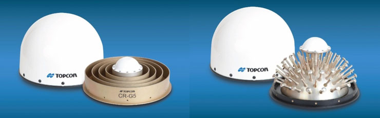
Left: Figure 6 – Topcon CR-G5-C antenna. Right: Figure 7 – Topcon PN-A5-C antenna.
The CR-G5-C antenna is of traditional Choke Ring type while the PN-A5-C antenna incorporates a convex impedance ground plane. Details of the PN-A5 antenna design and functionality could be checked with reference [4] below.A photo of cavity filters incorporated into a PN-A5-C and Topcon CR-G5-C antennas design is shown in Figure 8. A mechanical assembly outline of these antennas is shown in Figure 9 and Figure 10, respectively.

Figure 8 – Cavity filters incorporated into PN-A5-C and CR-G5-C designs
The mechanical design of the antennas is robust and shock resistant, but it is worth noting the internal space of PN-A5-C antenna allows for a larger filter to be incorporated. This results in improved protection against jamming and interference by this particular antenna.
Frequency response charts of Topcon PN-A5-C and CR-G5-C antennas are represented in Figure 11 and Figure 12, respectively. It is noteworthy that the GSM transmissions are suppressed by an amount of more than 80 dB. LTE and Inmarsat stations are suppressed more than 60 dB for PN-A5-C antenna and by about 40 dB for CR-G5-C. Additionally, the LNAs of these antennas have approximately a 50 dB gain. This is to compensate for longer cable runs normally used for reference station antennas. Such a high degree of interference suppression allows for the installation of the antennas in the close proximity to transmitting antennas of communication systems.
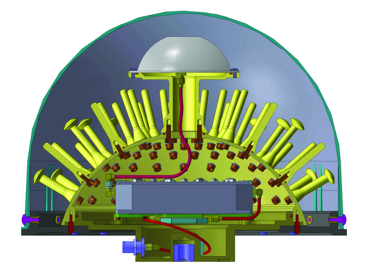
Figure 9 – Mechanical assembly of PN-A5-C antenna.
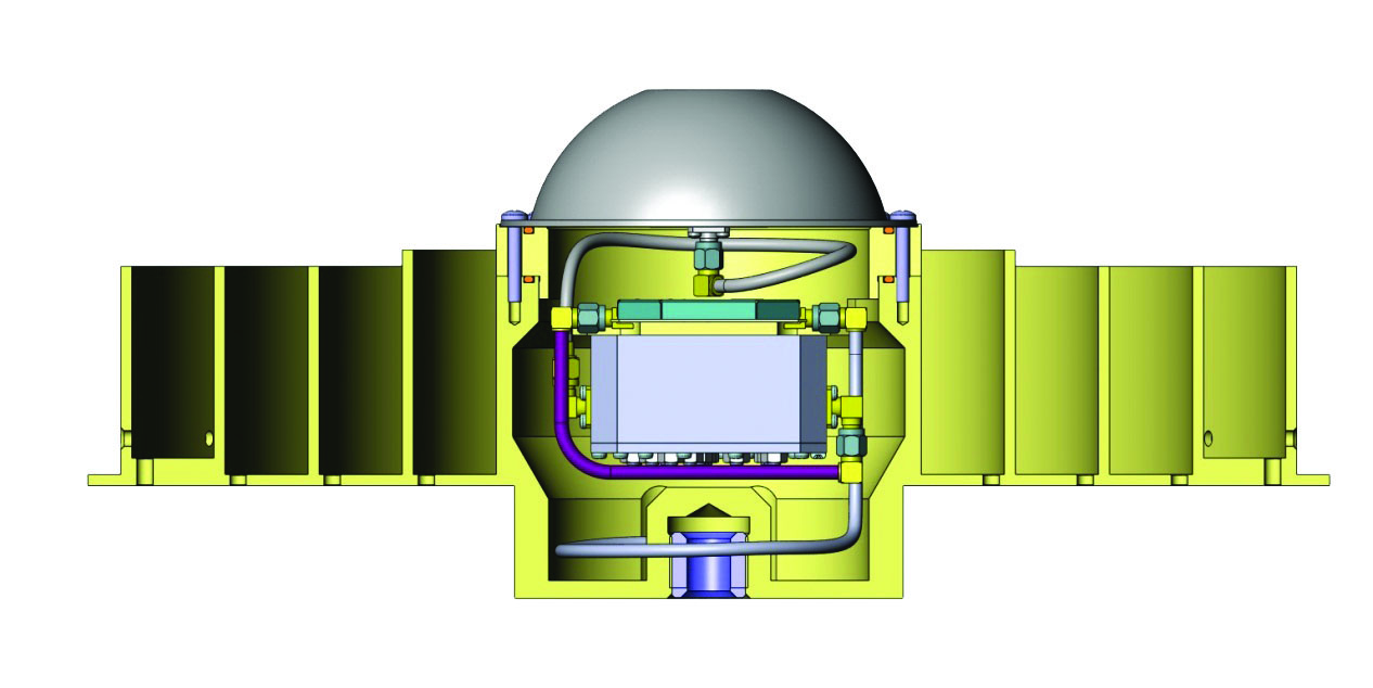
Figure 10 – Mechanical assembly of CR-G5-C antenna.
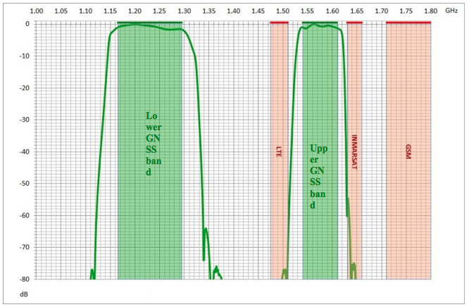
Figure 11 – Frequency response of PN-A5-C antenna.
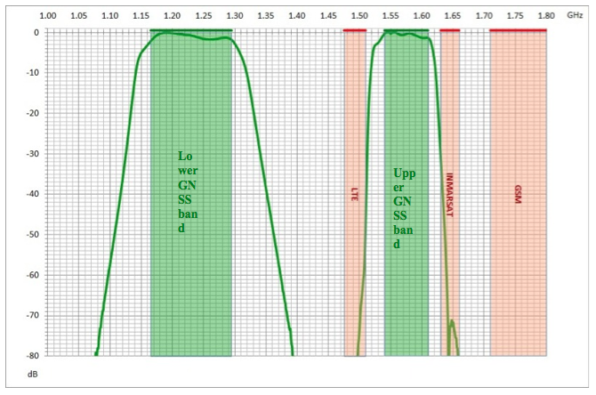
Figure 12 – Frequency response of CR-G5-C antenna.
References
- D. NatarajanA Practical Design of Lumped, Semi-lumped & Microwave Cavity FiltersSpringer, 2012
- J. Verdú, P. de Paco, Ó. Menéndez Microwave/RF Filters based on Bulk Acoustic Wave Resonators, LAP LAMBERT Academic Publishing, 2011
- Y.T. Lo (1993) and S.W. Lee (Editors) Antenna Handbook, vol.1 Fundaments and Mathematical Techniques, Chapman & Hall, New York
- D. Tatarnikov, Topcon PN-A5 GNSS antenna, part 1,2 Professional Surveyor, vol.32, issues 3,4, 2012