The Canadian federal government recently released the first new vertical datum in 80 years in Canada. The new vertical datum is called the Canadian Geodetic Vertical Datum of 2013 (CGVD2013). The introduction of this new datum not only establishes a more accurate and precise vertical reference system, it also introduces a new methodology for realizing elevations within Canada.
The CGVD2013 is now realized via the use of GNSS positioning methods along with a digital geoid model (the Canadian Gravimetric Geoid of 2013, CGG2013). What this means is that positioning professionals are no longer required to physically measure to benchmarks in order to establish a proper elevation within the CGVD2013. This is a drastic shift in the way in which elevations are established and will certainly take a significant amount of time before it becomes the de facto standard for determining elevations. (See the July issue of xyHt magazine for details.)
In order to properly realize an elevation at a particular point of interest, an accurate ellipsoidal height within the NAD83 (CSRS) datum first needs to be ascertained.
Next, the specific geoidal undulation (height between the NAD83 reference ellipsoid and the CGVD2013 geoid) needs to be determined for the point of interest. This is achieved by interpolating between the sample point data within the digital geoid model.
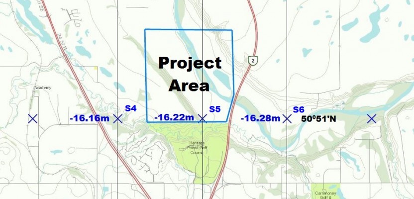
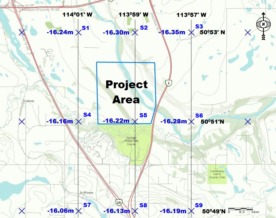
Last, the ellipsoidal height is transformed into an elevation by applying the geoidal undulation. The following example problem challenges you to perform a geoid model interpolation. This example uses the project area as shown in the figure below (click to view it larger).
Problem
Using the CGG2013 geoid model sample points shown in the figure, interpolate the geoidal undulation value for the point located at the NAD83 (CSRS) coordinates of 50∘ 51’45” N and 113∘ 58’20” W.
Solution Hints
1) Construct the L vector containing the geoidal undulations for the nine sample points.
2) Calculate the difference in latitude and longitude between the nine sample points, plus the point of interest, and the central sample point (S5) in units of decimal degrees.
3) Construct the A matrix.
4) Solve for the x vector containing the unknown polynomial constants (a0 … a8)
5) Generate the practical interpolation equation.
6) Substitute in the Xp and Yp coordinates for the point of interest into the practical interpolation equation and solve for the geoidal undulation.
7) Repeat step 6 for all other points of interest. This polynomial interpolation surface has a practical working range between 50∘ 50’ N and 50∘ 52’ N and 114∘ W and 113∘ 58’ W. Points of interest outside of this range should utilize a neighboring polynomial interpolation surface.