Identifying Blunders with Graphics

Mistakes and blunders are an inevitable part of being human. In fact, a wise person once told me that the only people who don’t make mistakes are those who don’t do anything.

Because a least squares adjustment of a plane survey is nonlinear, it will not arrive at a solution if a large blunder, such as a misidentified station, is present in the data. So, before we adjust our data, we must first remove any large mistakes. These can come in such forms as station misidentifications or recording and transcription errors.

As an example, in one of my early classes at Penn State, I had a group of students who were turning an angle eight times using the repetition method with a repeating theodolite. (Sorry young’uns, repeating theodolites were before your time on Earth.) While doing this they were also listening to a local radio station by the name of ROCK 107.

When it came time to average the accumulation of the eight angles, they proceeded to write in their field book that the angle was 107°. Of course, the angle wasn’t even close to 107°, but, obviously, the note-keeper heard the radio call sign of 107 at the same time he was recording the average angle.

This transcription error slipped all the way to the least squares adjustment where it was identified and corrected by reviewing the field notes. Fortunately, the use of data collectors today can help avoid this type of blunder, but many others can still occur. So, what methods can we use to identify blunders in our data and eliminate them?

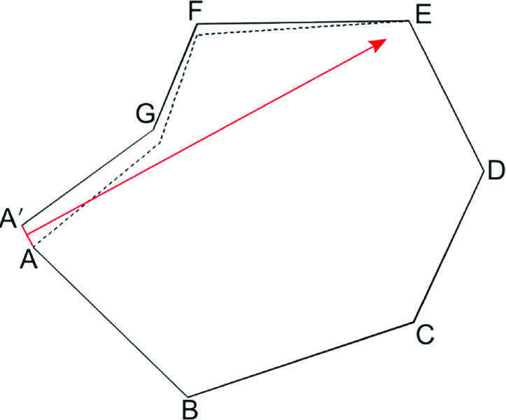
Figure 1: A traverse with an angle blunder

Graphical Methods

When a blunder occurs in a traverse survey, one of the first techniques that can be used to identify the blunder is graphical. To do this, plot the traverse in a CAD program using the raw observations. The misclosure line can then be used to help identify a single, large blunder in a traverse.

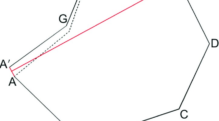
For example, assume an angular blunder is made at station E in the traverse shown in Figure 1. As shown in the figure, the dashed line represents the remaining traverse courses, which have been rotated by the angular blunder, resulting in a misclosure line AA’.

What the misclosure line now represents is the chord of the circle that was generated by rotation with the angular blunder at E. Thus, the perpendicular bisector of AA’ will point to the station with the angular blunder.

To verify that the angle at E has a blunder, assume coordinates for station E and assume an azimuth for the course EF, also.

When using this method it is important to use the raw observations and not adjusted angles, because adjusting the angles would spread the blunder to each of the angles in the traverse.

Proceed to compute the traverse as would typically be done using the raw observations again. When doing this, the angle at E is never used in the computations of the traverse misclosure. If the misclosure of the traverse is fine when starting the computations at station E, the angle at E definitely has a blunder and needs to be discarded or reobserved.

It should be pointed out that because there are other random errors in the observations, the perpendicular bisector will not point precisely to E but will appear to do so in the graphics software until you zoom in close on it.

The effects of a distance blunder are shown in Figure 2. The distance blunder will translate the remaining part of the traverse in the same direction as the course containing the blunder. In this case, a distance blunder occurred in line DE, which is shown as a dashed red line near Station E. This blunder translated the remaining part of the traverse such that the misclosure line AA’ matches the direction of DE closely, and its length matches the blunder closely.

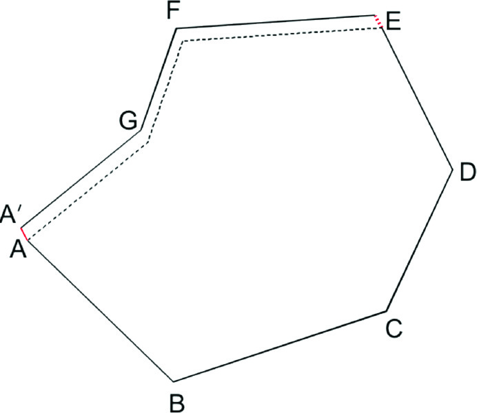
Figure 2: A traverse with a distance blunder

Thus, to identify the course with a distance blunder, find the course that most closely matches the forward or back azimuth of the misclosure line. Again, due to random errors in other observations, the direction and length of the misclosure line will not match the blunder in the course exactly, but they will be very close.

Unfortunately in this case, the course with the distance blunder must be reobserved to verify it is a blunder. Unlike angles, there is no mathematical procedure for verifying the blunder in the office with a simple closed traverse.

This speaks to the need to measure the distance of each course on both the foresight and backsight as you perform the traverse survey and to keep track of these observations separately so that a blunder can be identified. Today’s survey controllers provide options for this procedure and checks on backsights at each instrument setup so that such errors can be identified and removed at the time of their occurrence in the field.

For those of you who believe that distance blunders seldom occur, I relate the following evidence to the contrary. On the campus before our Academic Commons building was constructed, a property corner pin was visible at a distance of approximately 400 ft. from an NGS second-order monument, Hayfield SW.

Between the property corner and the NGS monument were two rows of crab apple trees. The lower branches of these trees prevented visibility of a normal rod with prism on the pin, so students would typically invert the prism on the property corner and observe the distance. In this position, the lay of the ground was such that the line of sight between the two stations was just above the grass.

We all should know that within a foot or two, the ground has a microclimate that refracts the line of sight.

Year after year, students would proceed in this fashion and end up with distances that were typically off by about a foot. I would send them back out where they would repeat the process, get a different length because of changes in atmospheric conditions, and again have a bad length for the course.

It wasn’t until I reminded them about the problem of a microclimate that they recognized what they had done incorrectly. Note that they had heard about the microclimate in earlier courses, but the information never seemed to sink in until they experienced it.

This may seem like a unique scenario, but I have seen students do the same thing near parked vehicles and buildings. In this case, the line of sight is close to the side of the object and again passing through a microclimate that refracts the line of sight.

In fact, my experience over the past 30 years of teaching surveying is that distance blunders occur more frequently than angle blunders because of the lack of field checks. Because you need to backsight your instrument anyway, always check your distance on the backsight, record it, and use it later as a second observation in a least squares adjustment.

This article looks at graphical methods that can be used to isolate blunders in observations. In the next article, I will present a simple statistical check on the residuals in the adjustment. Until then, happy surveying.