Part 1 of this article (March 2014) presents the differences between azimuths that surveyors observe with a total station and the geodetic azimuths listed in GNSS adjustment reports. However, the effect on angles caused by the deflection of the vertical at the observing station is typically small. Thus, the difference between the observed astronomic angle and geodetic angle is usually ignored. There is also difference between plane/grid azimuths and geodetic azimuths created by the convergence of the meridians.
In this article, I discuss the effect that convergence of the meridians has on traverse computations when geodetic azimuths are used. Unfortunately, this situation occurs more frequently today than in the past because GNSS adjustments often list the geodetic azimuths of observed baselines. Thus it is not uncommon to run a traverse between two stations that had their coordinates established by an earlier GNSS survey.
The coordinates and azimuths may also come from an NGS datasheet. When this occurs, some surveyors have used the computed GNSS baseline vector azimuths as their initial and closing azimuths for the traverse. However, when mixing geodetic azimuths with plane computations, the resulting angular misclosure can lead the surveyor to believe that either he made a large angular blunder in the traverse or the GNSS survey was in error or poor. In fact, it may be nothing more than the effect of the convergence of meridians. This, along with the fact that the second station used to establish the azimuths is often close to the traverse station, leads to large uncertainties for the GNSS-derived directions. 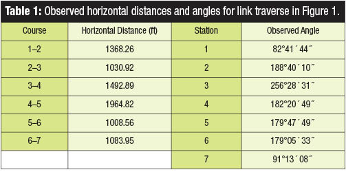 This article looks at the effect that both convergence of the meridians and accuracies of azimuths determined by a GNSS survey have on a conventional survey. It also briefly discusses the minimal effect that deflection of the vertical, as discussed in Part 1, has on the observed horizontal angles.
Convergence of the Meridians
A link traverse in Granite Bay, California is shown in Figure 1. It is considered closed mathematically because it starts and ends on two stations with known coordinates, which are typically listed in some map projection systems such as state plane coordinates. In Figure 1, Station 1 has California Zone 2 State Plane NE coordinates of (2,036,089.93, 6,804,070.13) ft, and Station 7 has NE coordinates of (2,033,593.21, 6,798,275.71) ft., both of which were obtained from a GNSS adjustment report. A link traverse also provides angular closure by having known azimuths to other stations at its starting and ending locations. 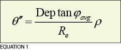 In Figure 1, a geodetic azimuth of 100°01′27.8″ was obtained from a GNSS adjustment for the line going from Station 1 to Az mk1. Likewise, the geodetic azimuth of 180°18′25.6″ was obtained from a GNSS adjustment for the line going from Station 7 to Az2. The remaining observed horizontal angles and horizontal distances are shown in Table 1.
In this case, we need to be concerned about convergence of the meridians because we are using geodetic azimuths to check angular misclosure. This is a problem because, unlike plane computations, all meridians, which are the reference directions, converge at the poles. Simply stated, all meridians, which are the due north in a geodetic sense, are not parallel as is assumed in plane computations. Thus, if a traverse goes east–west for what is a relatively short distance, the angular misclosure of a traverse will contain the difference between a plane north and geodetic north as part of the angular misclosure error when geodetic azimuths are used. In this example, the east–west distance of the traverse is only about 5794 ft, or about 1.1 mi.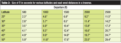 Recall from the September 2013 column, “Grid versus Ground,” that at every station there is a convergence angle. If we took the difference between the convergence angles at starting and ending stations, their difference would appear as part of the angular misclosure of the traverse. This error can be approximated by Equation 1 where θ″ is the difference between the forward and back azimuths of a line; Dep the overall departure, or east-west distance, of the traverse; ϕavg the average latitude of the traverse; Re the radius of the Earth where the average value of 6,371,000 m can be used; and ρ the conversion from radians to seconds, which is 206,264.8″/rad.
Table 2 shows the size of θ in seconds for various changes in departure in a traverse versus various latitudes in the conterminous United States. Note that the difference between the plane and geodetic north is smaller as we go farther south. If we traversed along the equator, this difference would be zero because all geodetic north are parallel along the equator. For the traverse in Figure 1 that has about 5800 ft in departure, θ″ is about 45.8″. 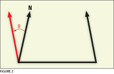 Thus, if we use two geodetic north from a GNSS adjustment to fix the direction of our traverse, we must take into account this difference when computing our angular misclosure for the traverse. This is because the forward and back azimuths in a traverse do not differ by exactly 180°, but rather by 180° ± θ.
A sketch, as shown in Figure 2, will often aid in determining the proper sign to the angular misclosure. However, if the traverse proceeds easterly the sign will be positive, and it will be negative when going westerly. Note in Figure 2 that the difference between the red and blue arrows shows the difference in azimuth of the line from its beginning to ending point.
If the azimuth for each course in the traverse in Figure 1 is computed with the given geodetic azimuths at the first and last station, we see an angular misclosure of −46.2″. This would cause most surveyors to stop and look at their angles for mistakes. However, almost 46″ of this is due to the fact that the meridians at the first and last station are not parallel. Taking convergence into account, the actual angular misclosure is only 0.4″. 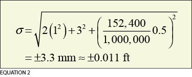 It would be a mistake to think that correcting the final azimuth for this convergence will then lead to a properly computed traverse. There is another theoretical problem that is present: the coordinates are based on the California, Zone 2, State Plane Coordinate System. As discussed in previous articles, the coordinates are based on grid azimuths, which are not parallel to geodetic azimuths except at the central meridian in the zone. So, while we can see that the angles do close acceptably when the convergence in the meridians is considered, this does not correct for the fact that the coordinates are based on an entirely different system in orientation.
To properly compute this traverse using plane computations, we must find the equivalent grid azimuths for both geodetic azimuths using the convergence angles at stations 1 and 7. Recall from the September, 2013 issue that we must also reduce the observed horizontal distances to their equivalent map project distances. Readers who are unfamiliar with these computations should refer to these articles.
If proper map projection computations are used, the traverse will close with a 1:66,000 relative precision and a linear misclosure of 0.12 ft. As stated in Part 1 of this article, the observed field angles should also be corrected for deflection of the vertical. However, this correction is often very small and ignored. In this traverse the correction to each angle ranges from −0.20″ to a +0.09″. This is true even with ξ and η deflection of the vertical components in the neighborhood of −5″ and −14″, respectively. Thus, this error would have little effect on the computational results.
A Word of Caution
Too often, too much significance is placed on azimuths that are listed in a GNSS adjustment report. That is, surveyors often assume these to be the exact geodetic values when, in fact, they can contain substantial amounts of error. This is not because the coordinates of the GNSS adjustment are poor but rather because the sight distance between intervisible stations is often relatively short.
For example, the manufacturer specifications for a static survey are typically given as 3 mm + 0.5 ppm today. For an RTK-GNSS survey, the errors are typically given as 10 mm + 1 ppm. These specifications are at 68% probability and ignore the setup errors of the receivers. To place these at 95%, we would need to multiply the overall error by about 2. To place them at 99.7%, we would need to multiply the overall error by about 3.
Assume that we can set up our receivers to within ±1 mm of the point. As was shown in the January article, this low of a value is unlikely; however, it still helps to demonstrate the problem. Further assume that our two intervisible stations are only 500 ft apart and that they are surveyed using the static surveying methods. The horizontal error in the each station in only 500 ft, or 152.4 m, can be computed in millimeters in Equation 2.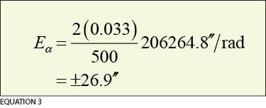 This error is relatively minor at 68%; however, when considering what will happen 99.7% of the time, this error is now ±0.033 ft at each station, which is still a small positional error but will result in a large uncertainty in the direction of the line. Since this error can occur at both stations, the error in the azimuth, Eα, between these two stations, which are only 500 ft apart, is Equation 3. Thus the error in the direction at a probability level of 99.7% is 80.7″.
 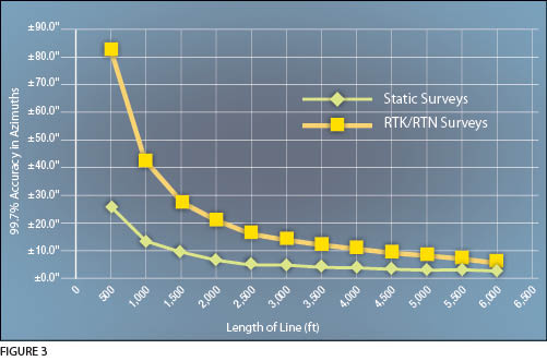 Figure 3 is a graph of the error in azimuth at a 99.7% probability level between two stations versus the distance between the two stations using the common GNSS static survey and RTK/RTN survey methods. Notice how the error in the azimuth is significantly large for a line less than 2000 ft in a static survey and how the accuracies begin to level off when observing lines that are greater than 2000 ft in length. Thus, use caution with directions from a GNSS survey when you’re performing a link traverse, because this uncertainty can and probably will appear as an angular misclosure error in the traverse.
Angular misclosure determined for a link traverse using geodetic azimuths can be significantly affected by the convergence of the meridians. This is true for even traverses that extend relatively short distances in the east–west direction. Additionally, the length of the line for a course whose azimuth has been determined by a GNSS survey can show significantly large errors when the length of the course is relatively short. These differences are also true between observed distances and their equivalent geodetic lengths. Since the inception of GPS in the 1980s, surveyors have seen distances listed in GNSS adjustment reports as either grid, geodetic, or mark-to-mark lengths. As we see in the next article, these values can differ significantly from the horizontal distances traditionally observed by a total station. Part 3 discusses the differences between geodetic, mark-to-mark, and horizontal distances.