Problems from using computed standard deviations.

According to the 2011 Minimum Standard Detail Requirements for ALTA/ACSM Land Title Surveys, “‘Relative Positional Precision’ means the length of the semi-major axis, expressed in feet or meters, of the error ellipse representing the uncertainty due to random errors in measurements in the location of the monument, or witness, marking any corner of the surveyed property relative to the monument, or witness, marking any other corner of the surveyed property at the 95 percent confidence level (two standard deviations). Relative Positional Precision is estimated by the results of a correctly weighted least squares adjustment of the survey.” (ALTA/ACSM, 2011)

In future articles I describe the error ellipses and their significance as a quality indicator of surveying observations. In this article l focus on the statement, “correctly weighted least squares adjustment of the survey.” In the previous article (November 2015), I discuss the use of the χ2 distribution to determine if the adjustment is weighted correctly or contains a blunder.

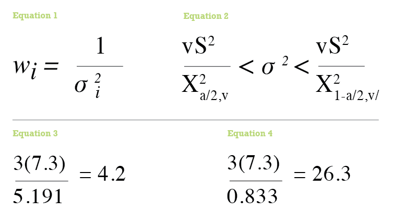
The real problem facing any surveyor is to decide how to assign standard errors of  σ1  to their observations so that the weights wi for the observations are appropriate for the errors present in the observations. Recall from the previous article that the weights for independent observations are computed as in Equation (1) where σ21 is the variance of the observation and σ1 the standard error of the observation.

In most commercial software sample standard deviations, S, are often used as substitutes for the standard error in Equation (1) because they are estimates of the standard error. But standard deviations are determined from a sample of data and not the population. As was shown in a previous article (November 2015), sample standard deviations or their variances can vary significantly from the standard error and variances of the population. This article demonstrates the problem that can occur by using computed standard deviations.

Problem?

Many surveyors will repeat the observations in the field, and their software will use standard deviations determined from the observations to compute the weights using Equation (1). However, surveyors seldom take more than four repeated observations with an angle and often even fewer in observing a distance. Because these are values computed from samples, they may not provide reliable estimates of their population values.

The X2 distribution.

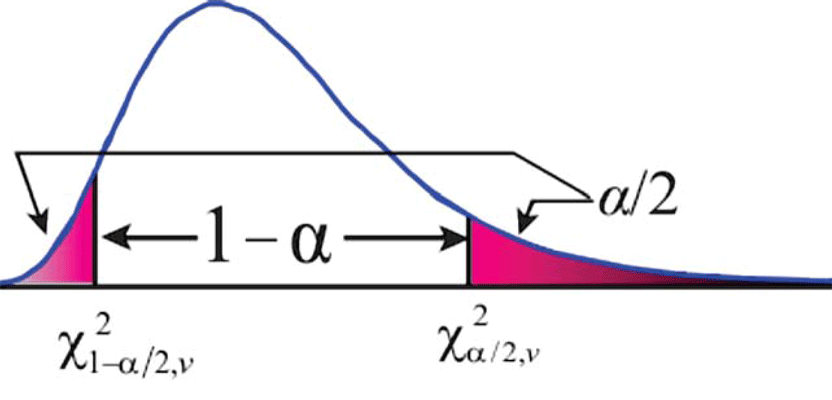
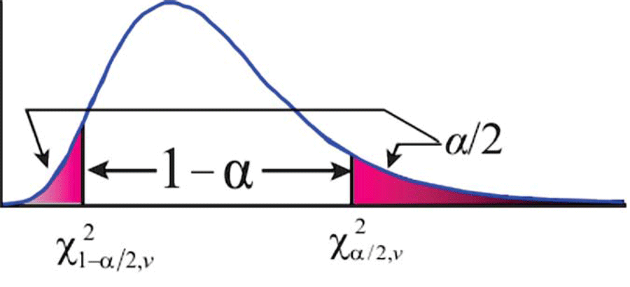
Fortunately, the χ2 distribution allows us to compute the range in which the population variance will reside at a selected level of confidence and provide some insight into the reliability of the sample standard deviations (Figure 1).

For example, assume that an observed angle has a sample variance of 7.3 (±2.7”2), which is computed from four repeated angle observations. The range that the population variance can be determined using critical values from the χ2 distribution is in Equation (2) where v is the number of redundant observations (which is three in this example), S2 is the sample variance (which is 7.3 in this example), and  χ2α⁄2 and χ21-α⁄2 are the critical values as determined from the χ2 distribution.

As we can see in Figure 1, the χ2 distribution is not symmetric like the normal and t distributions. Thus we need to determine the critical values for both tails of the distribution to obtain a range for the population variance at a particular (1 – α) probability.

We can get the critical values from the χ2 distribution by using statistical tables or using the chisq.inv() or chiinv() functions in spreadsheets. For example if we wanted the (1−α)% confidence interval, we could use chisq.inv(α/2,v) for the left-side critical value and chisq.inv.rt(α/2,v) for the right-side critical value in Excel.

In this example at 68.3% or one standard deviation, α/2 is approximately 0.158, χ20.158,3 determined using chisq.inv(0.158,3) is 0.833, and  χ20.158,3 determined using chisq.inv.rt(0.158,3) is 5.191. Thus the range for the population variance,  σ2i with a 68.3% confidence interval is somewhere between 4.2 (see Equation 3) and 26.3 (see Equation 4). This means that the proper weight for the observation is somewhere between 0.0014 and 0.56 range if units of seconds are used or between 61,486,928 and 2,390,368,806 if units of radians are used.

I should point out here that typically, in a least squares adjustment of a horizontal or three-dimensional survey, radian units are used for all angular values to avoid unit inconsistency with distance observations that are in English distance observations that are in English or SI units of measurement.

Not only is this a large range for the population variance and thus the weight that could possibly be used in the adjustment, but the sample variance is not from a truly independent set of observations. To obtain this value, the surveyor would need to reset the instrument and targets between each pointing or angle observation.

Stated another way: What is missing in the sample variance is the centering error of the instrument, the centering error of the target, and the leveling error of the instrument. While leveling error is typically only significant in cases where the line of sight is steep, the instrument and target centering errors tend to be the largest contributors to angular uncertainty with today’s instruments.

For example, when I was teaching I had second-year students perform eight repetitions of each angle in a braced quadrilateral. Sometimes the students could not complete the entire set of angles at a specific station in a single class period. Thus they would return the next week and reset the instrument and targets over the stations and complete their set of observations for the angles. This meant that they had to reset their targets and instrument over the stations. They would then compute the angular means and standard deviations for each set of observations. When they had to break their set of observations between class periods, they found that these standards deviations were much worse than those computed from a single setup. They often were troubled by this lack of accuracy and believed they had done something wrong.

However, I would point out that this higher value for the standard deviation was because they had setup errors included in their values and that these values were more representative of the actual uncertainties in their observations. Boundary surveyors often see these same errors in the resurvey of a property when they compare their observational values against the recorded values.

As previously stated, it is still common today to use sample standard deviations as estimates for the population standard errors when weighting observations in an adjustment. In fact, most software packages provide users with a default value entry to cover the possibility of the standard deviation being zero. This happens when all the repeated observations are the same and results in an invalid computation when entered into Equation (1).

So, you may be questioning: How do you actually get reasonable values for standard errors in order to “correctly weight” the adjustment? Well, the answer lies in estimating the setup errors and leveling errors and including these in the determination of the standard errors for the observations. I start this analysis in the next article of this series. Until then, happy surveying.