When planning GNSS control surveys on highway projects, it is important to understand the limitations of GNSS. Most highway projects are long, and linear distances that are wide open horizontally and vertically and are ideal for GNSS surveying. However, in rural and city areas, tree canopies and high-rise buildings will obstruct the GNSS signals, so a portion of the control survey must then be completed with a total station instrument.
One possible solution to adjust for the loss of open skies is to set GNSS control point pairs on either end of the project and then traverse with a total station through the tree obstructions and tie into the last two GNSS points. Depending on the length of the traverse and the orientation, a misclosure will ultimately result between the GNSS coordinates and the terrestrial ground coordinates. This is nothing to panic about but is simply the result of what is commonly referred to as the grid-to-ground correction.
The GNSS points are reduced to the state plane coordinate system by either post-processing the GNSS data or using GNSS-RTK capability in the field. Thus, even though the traverse begins and ends with two GNSS control points, the traverse distances are terrestrial (ground) and must be adjusted to the SPCS grid to check for misclosure.
Equation 1, Equation 2, Equation 3, Equation 4
Gathering the GNSS Data
A good example of grid-to-ground correction is a route survey performed in Georgia on a highway that was running due north for approximately 3000 feet. This traverse is an open-ended or a link traverse.
Two GNSS point pairs were set at the beginning and end of the survey. Fixed height 2-meter tripods were used for a static survey for two hours of occupation with Leica GPX1230 dual-frequency receivers. The data was post-processed in the office with Carlson Survey GNSS software and also sent to OPUS as a check.
Five traverse points were set between the GNSS control points, and angles and distances were recorded with a total station instrument with four direct and four reverse sets. The intermediate traverse points were turned in by a Leica total station and the elevations were determined by trigonometric leveling.
The beginning control points were numbered 500 and 501 and the ending control points were numbered 502 and 503. When finishing the field traverse with the total station, a quick inverse check with the data collector revealed a horizontal misclosure of 0.351 ft. between GNSS 502 and terrestrial point number 6 (502 and 6 are the same points).
When I returned to the office and downloaded the data into the survey software, I confirmed a horizontal misclosure of 0.351 feet. This results in a relative precision of 1 in 8400. Obviously, this is unacceptable for boundary surveys and is simply the result of the grid-to-ground correction. An adjustment must be made to bring the terrestrial (ground) coordinates into conformity with the GNSS grid coordinates.
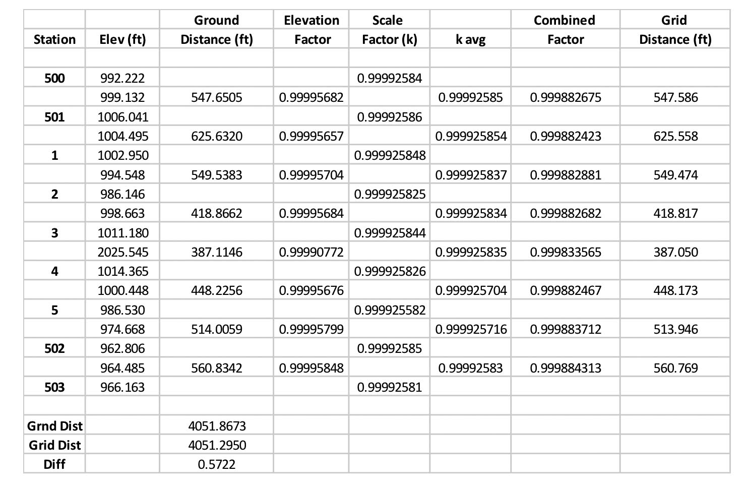
Table 1
Reducing Ground Distances to the Grid
Reducing ground distances to the grid is a two-step process:
- The ground distances must be reduced to the ellipsoid,
- then scaled from the ellipsoid to the developable surface or grid.
Because the area in question is approximately 3000-ft long, a simpler method can be used instead of more precise methods.
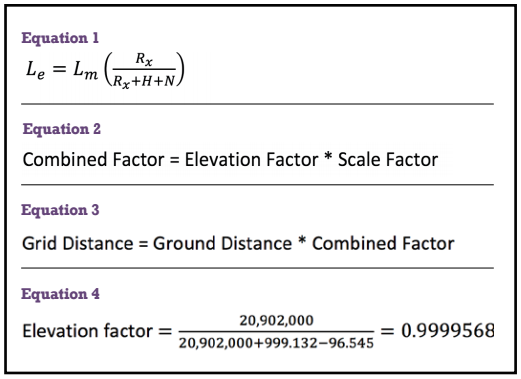
Equation (1) shows the computation for the ground surveyed length (Lm) and the ellipsoid length (Le) where:
- Rx is the average radius of the Earth (6,371,000 m or about 20,902,000 ft.)
- H is the average ortho etric height of the line (determined by GNSS post-processing)
- N is the geoidal height (determined by NGS GEOID12A)
This equation is a ratio, which is commonly called the elevation factor of the line. The next step in the process is to scale the ellipsoid length to its grid equivalent. In order to do this, a scale factor (k) is required, and this can be found by several sources. The latitude and longitude of a point can be entered into a state plane coordinate program, like the one at the National Geodetic Survey website, to retrieve the scale factor. Once the scale factor is determined for each point, an average is then taken for each line.
In Table 1, the average orthometric elevation is determined for each line and the distances displayed are ground. The elevation factor is determined by Equation (1). The scale factor is determined by entering the latitude and longitude of each point into the program provided by the National Geodetic Survey’s website (the SPC toolbox at ngs.noaa.gov/TOOLS/spc.shtml contains the conversion software that provides the scale factor at a point). The geoid height, N, can also be determined from several sources including software on the NGS website.
Then, each individual value is entered into the elevation factor equation, even though an average N value would be sufficient. The average scale factor is then determined for each line. Equations (2) and (3) round out the last two columns of the spreadsheet in Table 1.
As an example, the average elevation of stations 500 and 501 is 999.132 ft. The average geoid height for the stations, which was obtained from Geoid12B on the NGS website, is 96.545 ft. Thus the elevation factor for the line is as shown in Equation (4).
Using the SPC software on the NGS website and the latitude and longitude of the points 500 and 501 from the GNSS survey, the scale factor (k) for point 500 is determined to be 0.99992584. Similarly, the scale factor for 501 was determined to be 0.99992586. The average of these scale factors is 0.99992585.
The combined factor is then determined as 0.99995682(0.99992585), which yields 0.999882675. This combined factor is then multiplied by the observed horizontal distance to get the grid distance 547.586 ft., or 0.999882675(547.651) = 547.586 ft. This process was continued for each observed horizontal distance.
It is important to note that control points 1 through 5 were turned in with a total station and are therefore ground coordinates. GNSS values could not be obtained for these control points due to tree obstructions. Thus, coordinates for these locations were treated as GNSS points to gather Geoid values and are therefore approximate.
Equation 5, Equation 6
The Final Adjustment
The difference between the overall ground and grid distances is 0.572 ft. Also, the original misclosure was 0.351 ft., resulting in a precision of 1:8400. Entering the scaled distances (grid distances) into a new compass rule adjustment, holding the original azimuths, and then processing the new distances results in a linear misclosure of 0.006 ft., with a relative precision of 1:717,800.
Most surveying software available today can reduce and adjust this survey. One must keep in mind that the ground distances were scaled to the grid. The GNSS SPCS coordinates are on the grid, and now the observed horizontal distances are in the same grid system.
This high relative precision reveals the fact that the control traverse was very tight, and this can be attributed to very good field procedures by experienced field technicians, adjusted tribrachs, and a calibrated instrument. Systematic errors can be reduced by balancing the foresight and backsight distances and turning multiple sets of angles.
Now that the control is adjusted, the topographic survey can begin. In order to keep all distances on the grid, a combined factor must be entered into the data collector. The combined factor can be an average value that represents the middle of the project, and this is more of a subjective decision on the surveyor’s part.
Because the control was running due north, the convergence angle was negligible in this adjustment process. However, the difference in convergence angles for the endpoints will come into play if the traverse runs in an easterly or westerly direction.
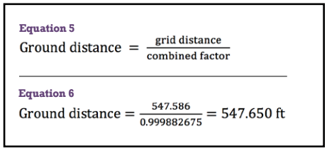
One must also keep in mind that in order to follow in the footsteps of the original surveyor, the boundary distances must be ground. Therefore, this survey is an example of a specific requirement that all coordinates remain on the specific state plane coordinate grid system determined by the client. A good example is a municipality that requires a topographic survey for aerial mapping. In order to convert the adjusted grid coordinates back to ground distances, Equation (5) can be used.
For example, assume the adjusted grid distance for the line between 500 and 501 is 547.586 ft. The adjusted ground distance is then computed as in Equation (6).
The next article will discuss an open (link) survey that runs in an easterly direction whereby the difference in the convergence angles at the endpoints is applied to adjust the survey. I would like to thank Dr. Charles Ghilani for his assistance in writing this artcle. Dr. Ghilani is an invaluable resource to the geomatics profession worldwide.