The t Distribution, Part 2

In the previous article (July 2015), I introduce the concept of sampling distributions and the need to use these distributions to analyze small samples of data. In surveying, observing small samples is typical where angles are often observed only two or four times, and repeated distance observations simply means pushing the measure button more than once. Sampling distributions are based on a sample’s mean and variance as well as the number of redundant observations known as its degrees of freedom.

The degrees of freedom are all the observations made beyond what is necessary to determine a value. So, for instance, if we made four observations of an angle, any one of these values could be used to state the size of the angle. The remaining three additional observations are considered redundant observations and represent the degrees of freedom for the observation.

Obviously, these additional observations are used to remove systematic errors, check the first observation, and create a mean and standard deviation for the angle. This sample is said to have three degrees of freedom that represent these additional observations.

As the number of redundant observations increases, the critical values from the sampling distribution approach the values for the same confidence level from the normal distribution.

For example, at 30 degrees of freedom, the critical value from the t distribution is 2.04, which is not far from its normal distribution value of 1.96. Note that the t distribution becomes the normal distribution with an infinite number of observations.

In the past the only way to determine the critical values for a distribution was to have access to a statistical table. However, today spreadsheets provide this capability with built-in functions.

For example, in Excel the function to determine a critical value for the t distribution is tinv (α,v) where α represents the level of confidence and v represents the degrees of freedom. So in the aforementioned scenario, it would be tinv (0.05,3) where α is 0.05 (95% probability level) and 3 is the number of degrees of freedom in the sample of four observations as previously discussed. [Note that Microsoft Excel requires the entry of 0.05 for the critical t value (t_0.025,v). This is not the case with other distributions.]

In this case the critical value, our multiplier for a 95% confidence interval, is 3.182… This value is far different than the value of 1.96 derived from the normal distribution. This value is greater simply because our sample size is small, and thus there is more uncertainty in the mean and standard deviation than was determined from the sample of observations.

Recall that in a previous article on the normal distribution (June 2015) I state that multipliers from this distribution are valid only if we observe more than 30 repeated observations. Since this seldom happens in surveying, we need the t distribution to analyze our data for outliers and blunders.

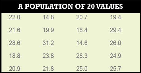
Table 1

Here I look at how the t distribution can be used to perform this analysis. To show this, Tables 1 and 2 from the previous article are repeated here.

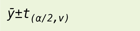
As an example, using line 1 in Table 2, we can state that 95% of the time the population mean will be between what’s shown in Equation 1 where ȳ is the mean for the sample, S the standard deviation for the sample, n the number of observations made, and t the critical value from the t distribution for α percentage points based on a sample with v degrees of freedom.

Note in this equation that S/√n represents the standard deviation in the mean, which is used to determine a range for the population mean. If we wished to determine a specific range for a single observation, we would replace this with the standard deviation for a single observation, S.

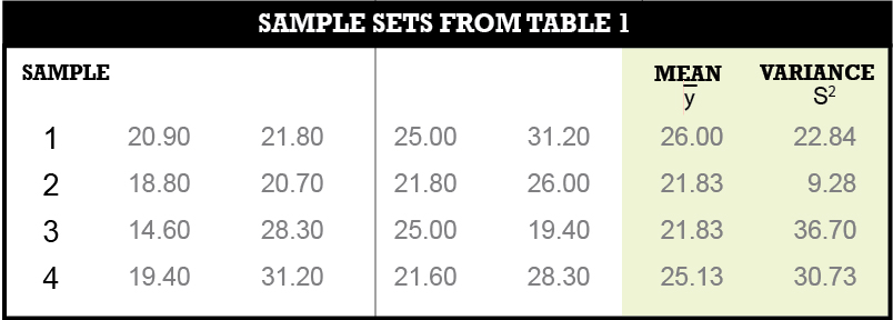
Table 2

In this example the mean is 26.00, the standard deviation equals √22.84, n equals 4, α equals 0.05, which is 1 – 0.95, and v equals 3, which is the number of redundant observations. Thus the 95% confidence interval for the population mean based on these samples’ values is as shown in Equation 2.

The t value for a sample with 3 degrees of freedom is 3.183, which is considerably larger than the 1.96 (or 2) multiplier that would be used from the normal distribution. This larger multiplier represents the uncertainty we have in the mean and standard deviation from the sample due to the limited number of observations used to determine these values.

Thus, we can state with 95% certainty that the mean for the population is between 18.39 and 33.60, which also means that 5% of the time the population mean will be outside this range.

Equation 1

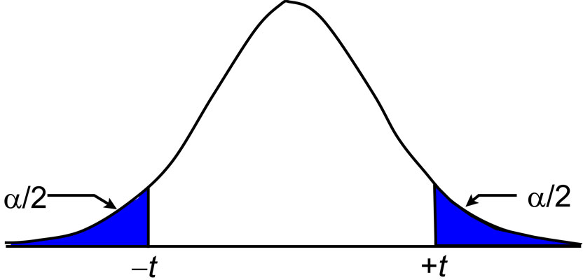
A more common use for this distribution is to determine the range in which 95% of the observations should lie. This is typically used to identify and remove outliers or blunders from the observations. Thus we are stating when we do this that we are willing to discard 5% of our observations as possible blunders, which is why 99.7% is sometimes used.

For example, assume that a distance was observed four times and had a mean of 293.56 ft with a standard deviation of ±0.023 ft. In this case 95% of the observations should lie between 293.56 ± t_0.025,3(0.023). Since the t multiplier is again 3.183, this means that 95% of the observations should be between 293.487 and 293.633.

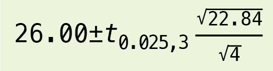
Equation 2

If any observation is outside of this range, it could be considered a blunder or outlier and discarded from the sample. Again, this means that we are willing to discard 5% of our observations in order to remove any possible blunders.

Often the survey controller will display the mean, its standard deviation, and the residuals when multiple observations are made on a quantity. In this case, the product of the t value and the standard deviation of the observation provide the range/confidence interval for the residuals. Using the previous example, 95% of the residuals should be between 3.183(0.023) or ±0.073 ft.

It is important to remember that when we are surveying, we generally collect very small samples for our observations. Thus, the sample means and standard deviations have higher levels of uncertainty than those derived from the normal distribution, which comes from an entire population of observations. Unless we collect more than 30 samples of a single value, we really should be using the critical values and multipliers from the t distribution and not the normal distribution.

In the next installment, I explore the use of the Chi-squared (χ2) distribution, which is used to develop the “goodness of fit” test in least squares adjustments. In particular, I look at the use of the distribution, what “failing the test” means, and what to look at when the test does fail.

Until then, happy surveying.