Part 2: The Normal Distribution
Part 1 of this series appeared in the May 2015 issue.Errors in observations can be classified as systematic or random.
Systematic errors follow physical laws and can be mathematically corrected or removed by following proper field procedures with instruments. For example, the expansion or contraction of a steel tape caused by temperatures that differ from the tape’s standard temperature is a systematic error that can be mathematically corrected.
Often in surveying we correct for systematic errors using the principle of reversion. For example, we can compensate for the vertical axis of a theodolite not being perpendicular to the horizontal axis by averaging angles observed in both the face I (direct) and face II (reverse) positions. We remove the effects of Earth’s curvature and refraction and collimation error in differential leveling by keeping our backsight and foresight distances balanced between benchmarks.
Of course, mistakes (also called blunders) are a fact of life because we are human. (A wise man once told me that the only people who never make a mistake are people who never do anything.) Mistakes are not errors but must be removed from our data. These can range from simple transcription errors to misidentifying stations to improper field procedures. Mistakes can be avoided by following proper field procedures carefully.
There is no theory on how to remove a transcription error other than to catch it at the time of occurrence or hopefully later in a post-adjustment analysis.
Random errors are all the errors that remain after systematic errors and mistakes are removed from observations. Random errors occur because of our own human limitations, instrumental limitations, and varying environmental conditions that affect our observations. For example, our ability to accurately point on a target depends on the instrument, our personal eyesight, the path of our line of sight in the atmosphere, and our manual dexterity in focusing the instrument and pointing on the target. As another example, an angle observation depends on the ability of the instrument to read its circles in this digital age and the ability of the operator to point on the target.
In fact, all manufacturers have technical specifications for their instruments that indicate the repeatability of the instrument in an observation. For example, the International Organization for Standardization (ISO) 17123-3 standard, which replaced the DIN 18723 standard, expresses the repeatability of a total station based on specific procedures in the standard. These standards were devised to help purchasers differentiate between the qualities of the instruments. They were not meant to indicate someone’s personal ability with an instrument because the pointing error is a personal error.
As an example, every year I had second-year students replicate the DIN standard to determine their personal value for a particular total station. Some students would obtain values that were better than the value published for the instrument, others would get values very close to the published value, and some would get values greater than the published value. These variations depend on their personal differences.
No matter whether we are using total stations, automatic or digital levels, or GNSS receivers, the random errors from observations we collect will follow the normal distribution curve. The normal distribution is based on an infinite amount of data. Thus, it is not appropriate for polls performed for elected officials because the voting public is a finite number.
However, in surveying, we could spend our entire life measuring one distance, followed by our offspring’s lives, and their offspring’s lives, and so on forever trying to determine this single length. No one is suggesting we do this. However, when we take a sample of data for an observation, the sample is from an infinite number of possible observations and follows the normal distribution and its properties. In fact, observational errors in astronomy were the reason for the creation of the normal distribution and least squares.
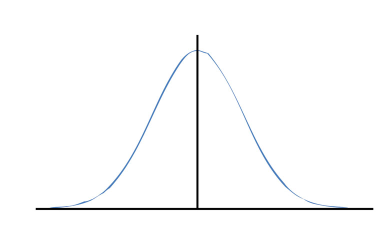
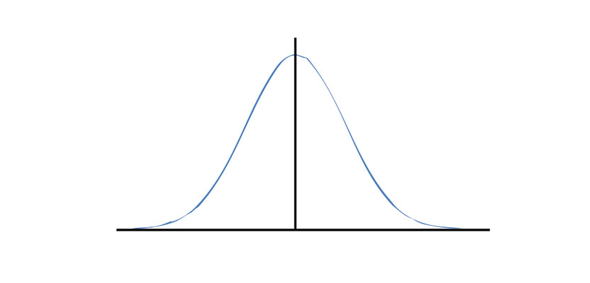
Figure 1
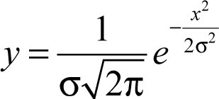
Equation 1
As shown in Figure 1, normally distributed data is symmetric about the center of the data. The ordinate (y coordinate) of the distribution is defined by the Equation (1) where σ is the standard error of the population and x is the size of the error. Thus x represents the residuals for each observation with the center of the curve at zero.
As can be seen in this figure, most errors are grouped about the center, but some large, random errors can and will occur. What we need to do as surveyors is find these large random errors and mistakes and remove them from the set of observations. This can happen in the field, before the adjustment, or in a post-adjustment analysis. In fact, one of the advantages of using least squares adjustment is the fact that it is possible to statistically analyze the residuals and determine when a residual is too large.
Isolating Mistakes and Outliers
The area under the normal distribution curve shown in Figure 1 is always equal to 1. This curve is asymptotic (comes close but never touches) the x axis.
What the first statement means is that 100% of the data lies under the curve. What the second statement means is that large random errors can occur but seldom do. Additionally, there should be as many observations with negative residuals as there are with positive residuals.
Another fact of the normal distribution is that slightly greater than 68% of the residuals should lie within one standard deviation of the mean which is at the center of the curve. That is, about 68% of the residuals should lie between y̅– S andy̅+ Swhere y̅is the mean of the data, and S its standard deviation.
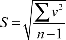
Equation 2
The standard deviation is computed as shown in Equation (2) where v represents the residual of a single observation, which is defined as v = y̅– observation, and ∑v2 is the sum of all the observational squared residuals. If you are wondering why squared, it is because the simple sum of all the residuals is always zero excepting rounding errors. Thus the interval y̅± S should contain about 68% of the observations when we make repeated observations.
If we were willing to call 32% of the observations as blunders or outliers (recall outliers are large random errors), we could discard or re-observe all observations that fall outside this 68% interval. However, if we did this, we would soon be out of business. Most surveying standards are based on a 95% interval. In blunder detection often 99% or greater is used. The reason is that we are willing to accept an error that is outside this interval is more likely a blunder (mistake) than a large random error (outlier).
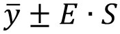
Equation 3
To determine the 95% confidence interval we need a multiplier. That is, the 95% interval for a set of data is given as shown in Equation (3) where the multiplier is E. Table 1 shows various multipliers for selected probabilities. In practice, it is common to use an interval of two times the standard deviation to determine those observations that are considered blunders. This value of 2, which should be 1.9599, comes from the normal distribution where 95% of the residuals are centered on zero in the normal distribution.
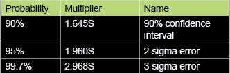
Table 1
This brings up another interesting fact in statistics: it is okay to say that 95% multiplier is 2 rather than 1.9599 or 1.96 because in statistics this will make little difference in the actual analysis. In fact, I like to say that statistics are a little fuzzy.
As an example, Table 2 shows 15 distance observations (Obs.) for the same course. The mean for this data is shown in Equation (4). Using this mean, the residuals computed for the observations are in the columns following each observation. The sum of the squared residuals is 0.077735. Substituting this value into the equation for computing S yields the standard deviation for a single observation of about ±0.074. The 95% interval for the set of observations is 212.237 ± 1.96(0.074) resulting in a 95% range between 212.091 and 212.383.
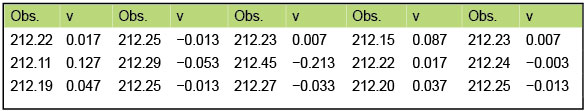
Table 2
Looking at the data in Table 2, we see that the distance 212.45 is outside this interval. It would also be outside the 95% range if a multiplier of 2 had been used. Thus, this observation can be discarded from the set as either a large random error or a mistake. By doing this we have used one of the properties of the normal distribution to isolate an observation for removal from a set of data.

Equation 4
It is interesting to note that even in this set of observations, there are 7 negative residuals and 8 positive residuals. Given that the set of data has 15 elements, this data does adhere to one of the basic principles of normally distributed data in that the observations are evenly distributed about the mean, or as even as 15 observations can be.
However, some of you may realize in the above example that there are only 15 observations and that the normal distribution is based on a population of data with an infinite number of observations. Still, 15 observations for a single distance is more than any surveyor will collect typically. While the principles derived from the normal distribution are true, we never collect an infinite set of data and seldom more than 30.
In a later article, I will discuss how we can perform a similar technique with a small sample of data using a sampling distribution.
Until then, happy surveying!