Educate: Where Theory Meets Practice
In previous articles I’ve discussed the reduction of conventional surveying observations to their geodetic equivalents. This article presents how these observations can be reduced to simple vector components that match GNSS surveyed baseline vectors. Unfortunately this transformation of conventional observations to GNSS baseline vectors involves three-dimensional rotations, so the mathematics will increase.
As shown in Figure 1, when we set up on the surface of the Earth we establish a local coordinate system (NEU) that is not aligned with the geocentric coordinate system that GNSS satellites use. This local system has axes for geodetic north (N), east (E), and up (U), where up is defined by the direction of the normal through this point. Thus U is defined by the perpendicular to the ellipsoid and not the geoid.
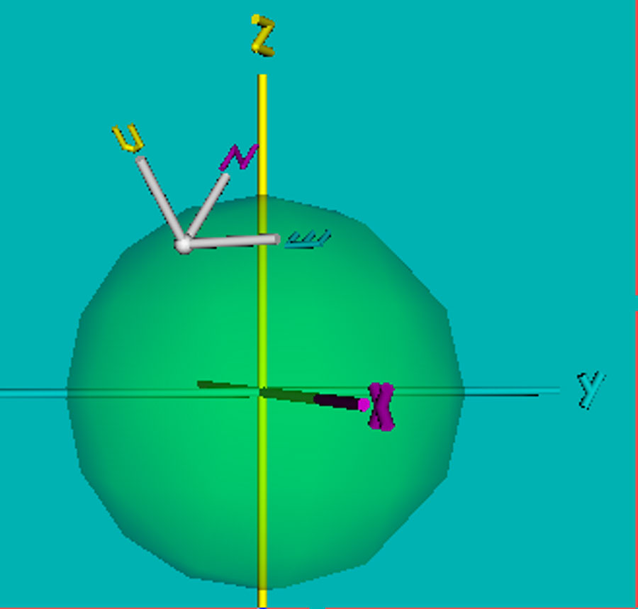
Figure 1
If our angle observations have been reduced to their equivalent geodetic observations (see the March, 2014 issue of Professional Surveyor), this is known as the local geodetic coordinate system. When the observations are not reduced, it is known as the local astronomical system. The local geodetic coordinate system has its origin at the center of the instrument with north being the x axis and east being the y axis. Unfortunately, this definition creates a left-handed coordinate system.
The positive direction of the axes in a coordinate system can be determined by viewing the axes using your hand—thus, the names left-handed and right-handed coordinate systems. Figure 2 depicts the formation of a right-handed coordinate system, which is traditionally used in mathematics. As seen in this figure, the thumb points in the direction of the positive X axis, the first finger points in the direction of the positive Y axis, and the second finger points in the direction of the positive Z axis.

Figure 2
In a left-handed coordinate system, the positive X axis points in the opposite direction of a right-handed coordinate system. The positive end of an axis is important in determining whether we need a positive or negative rotation.
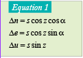
Figure 3 depicts the changes in neu coordinates as derived from the slope distance s, azimuth α, and vertical angles z or v of a course between two stations. Using the geodetic zenith angle z, geodetic azimuth α, and the slope distance s between two stations, changes in local geodetic coordinates can be computed as shown in Equation (1).
 However when the instrument is moved from its location, the origin of the local geodetic coordinate system also moves, and thus a new coordinate system is created. Of course, this is not ideal. Thus we need to convert these coordinate changes that actually define a vector similar to a GNSS baseline vector into a recognized coordinate system.
A coordinate system already used by GNSS receivers is the geocentric coordinate system. This coordinate system, shown in Figure 1, is commonly referred to as an earth-fixed, earth-centered coordinate system because its origin is at the mass center of the Earth. The orientation of its Z axis is defined by the conventional terrestrial pole (CTP) of the Earth (as defined in 1984); its X axis is defined by the intersection of the Greenwich Meridian (GM) with the equatorial plane; and its Y axis is placed in the equatorial plane to create a right-handed coordinate system.
This type of coordinate system is used to define GNSS baseline vector components. Thus if we can rotate the coordinate changes from the local geodetic coordinate system into the geocentric coordinate system, we will generate coordinate changes that match GNSS baseline vector components of (ΔX, ΔY, ΔZ).
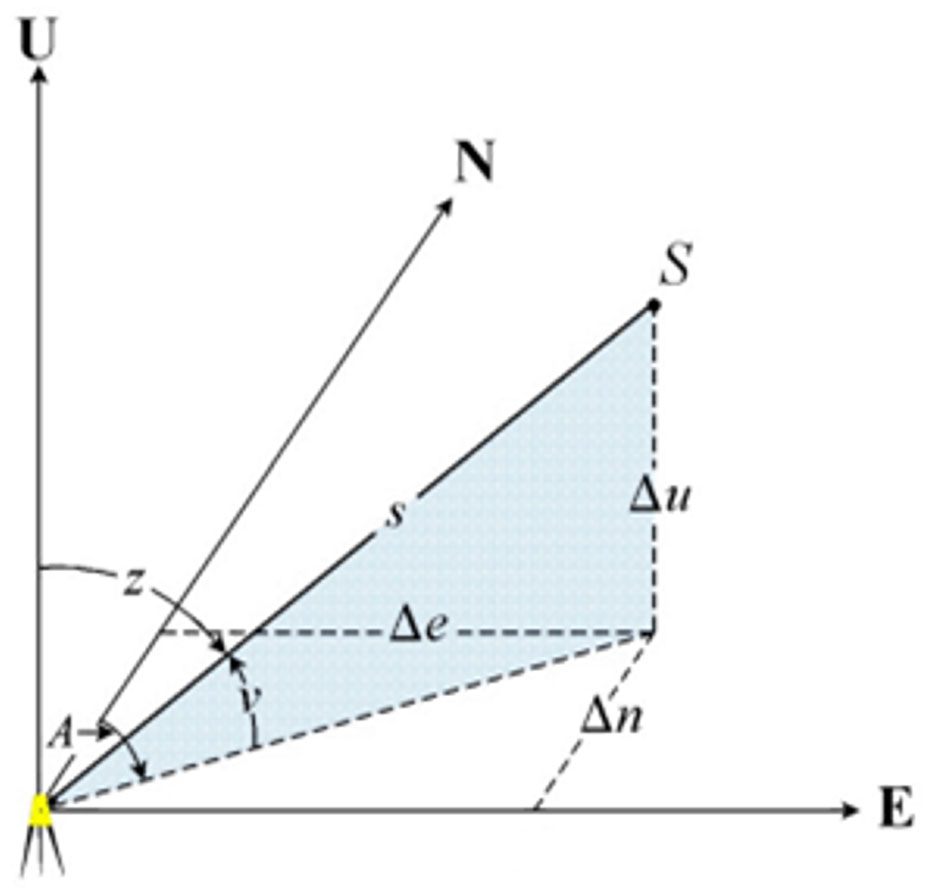
Figure 3
Rotations
We need to perform a series of rotations to convert the local coordinate changes into GNSS baseline vector components. Figure 4 depicts the rotation of a XY2 axis into a XY axis coordinate system. In this coordinate system imagine the positive Z axis being perpendicular to the page and coming up at you. In this case a positive rotation is a counter-clockwise rotation as shown in the figure.
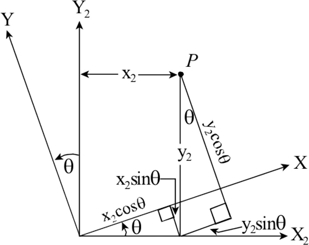
Figure 4
The goal is to convert the (x2,y2) coordinates into (x,y) coordinates by rotating the entire system about its Z axis. To view this rotation, put your right
hand in the configuration of (c) in Figure 2, point your second finger at your face, and then rotate your hand counter-clockwise. This rotation will convert the coordinates from the X2Y2 coordinate system into the XY system.
The mathematics for this rotation is as follows. Noting the x2 coordinate is the hypotenuse of the right triangle at the bottom of the figure with its adjacent side lying on the X axis and further noting that the y2 axis is the hypotenuse of the right triangle in the right side of the figure with side opposite P on the X axis, we can see that the x coordinate of point P is the sum of the side adjacent to the rotation angle in the first triangle and the side opposite the rotation angle in the second triangle, or Equation (2).

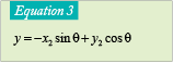
Similarly, the y coordinate can be determined by subtracting the side opposite the rotation angle in the first triangle from the side adjacent to the rotation angle in the second triangle, or Equation (3).
Since the z coordinate is not being rotated, the transformation of the z2 coordinate is simply as shown in Equation (4).
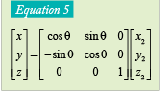
The complete three-dimensional rotation can be expressed in matrix form as shown in Equations (5).
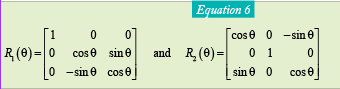
Since this rotation is about the Z axis, this is known as the R3 rotation. Similar rotations can be defined about the X and Y axes, which are known as the R1 and R2 rotations, respectively, and can be written in matrix form as Equation (6).
The rotation angles necessary to take the changes in local geodetic coordinates shown in Equation (1) into a conventional terrestrial system, such as WGS84, can be determined by looking at the geometry in Figure 5.
Figure 5(a) depicts the local geodetic coordinate system in relation to a conventional terrestrial coordinate system. The first rotation that is required is to rotate the ne plane so that it is parallel with the XY plane. As shown the amount of rotation required is 90° − latitude (φ) of the location where the instrument is setup. This rotation is about the e axis and clockwise, so a positive rotation angle θ is φ − 90° using a R2 rotation, since the e axis corresponds to the y axis in this left-handed coordinate system.
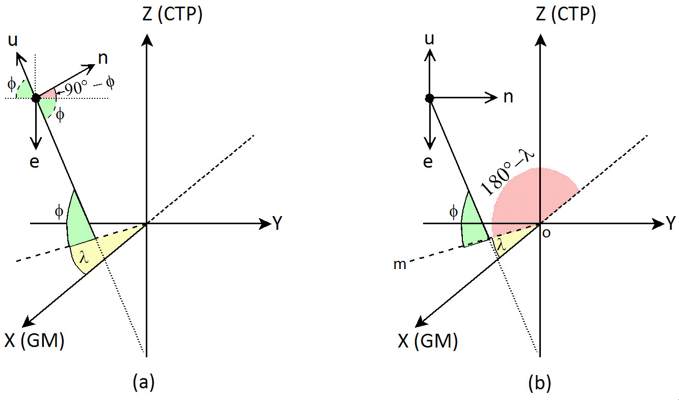
Figure 5
After this rotation is completed, the once-rotated local geodetic coordinate system will look like that shown in Figure 5(b). Note that the northing axis was originally pointing at the pole (CTP). After the first rotation it will still be pointing at the polar axis oZ and is therefore aligned with the line mo drawn in the equatorial plane. If we simply did a 180° rotation about the u axis, which is a R3 rotation, the positive n axis would then point to m. However, we need it to align with oX.
As shown in Figure 5(b), this rotation is simply 180° − λ about the u axis. Again, this is a clockwise rotation when viewed from the positive end of the u axis and thus a negative rotation. Therefore, the positive R3 rotation for θ is λ − 180°.
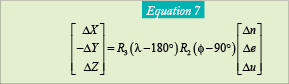
If you have been following the rotations, this leaves the twice-rotated easting pointing in the direction of the negative y axis. By simply changing the sign of the twice-rotated easting coordinate, the original left-handed coordinate system can be converted into a right-handed system. Thus to take the changes in the neu coordinates into a conventional terrestrial coordinate system, we need to perform the following sequence of rotations as shown in Equation (7).
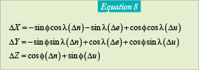
Substituting the appropriate rotations and making the appropriate trigonometric substitutions completes the equations as shown in Equation (8).
At this point, assuming you have read this far, we can now take observations from the field, convert them to their geodetic values, and rotate them into a recognized coordinate system. This method provides one way of combining GNSS and conventional observations. In fact, the software you purchase with your GNSS receiver may do these conversions or very similar ones many times in a typical project.
 However, there is another method that brings GNSS baseline vectors into any local coordinate system, assumed or otherwise. Instead of working in the GNSS reference system, it is possible to create a map projection that brings the GNSS observations to the surface. This involves creating a low-distortion map projection for your project.
A low-distortion map projection is created when the developable map surface is at or near the surface of the Earth for your project. Thus the distance observations will not need to be reduced and will nearly match those provided by your GNSS software. Additionally, the map projection needs to be conformal to preserve the angular observations.
The next article will discuss this method of bringing your GNSS observations in agreement with observations made with conventional instruments. Until then, happy surveying!