In my previous article in the September issue, I demonstrate one method of taking conventional/optical observations and converting them into GNSS baseline vectors. Here I demonstrate how to create a map projection system that is near the ground, and thus on the surface we survey. These map projections are commonly referred to as low-distortion projections; however, they are simply map projections designed on or near the surface of the Earth. They work best where elevation differences are not too great and the area covered by the map projection is also relatively small. However, they can be designed to fit locations with moderate elevation differences. (For an article about a Pennsylvania low-distortion project by James A. Wyatt, see xyHt.com.)
Low-Distortion Map Projections
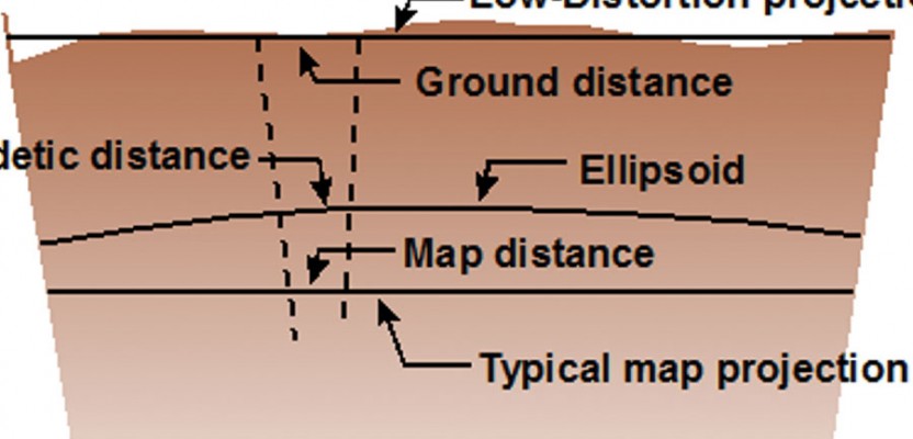
The advantages of low-distortion projections are that the grid distance determined by the inverse of the coordinates between points will closely match the observed horizontal distance. The figure here demonstrates how this is possible.
Map projections, such as the ones used for state plane coordinate systems, are designed to minimize the distortion between a geodetic distance on the ellipsoid and a distance on the map projection surface. Unfortunately, we work on the surface of the Earth, and thus the elevation of the project can often result in large distance distortions.
 For example, Flagstaff, Arizona at 7,100 feet has an elevation factor of 0.99966, which results in a distance precision that is less than 1:2400 when a grid distance is compared to an observed horizontal distance. However, if the map projection surface is placed at or near the average elevation of the project, this will virtually eliminate distortions to distances caused by their elevation. Of course, the last statement assumes that elevations in the region covered by the low-distortion projection do not vary too much.
Additionally, as can be seen in the figure, the typical map projection system, such as those used in state plane coordinate systems, creates a second scale factor that is needed to reduce the geodetic distance to the mapping surface. Most state plane coordinate zones limit the distortion between the geodetic and map distance to 1:10,000. This value was sufficient in the 1930s when the measuring tools were a steel tape and transit but is insufficient for today’s instruments. However, the value of 1:10,000 was necessary to allow the state plane coordinate zones to cover a large region. Even so, large engineering projects seldom cover such expansive areas.
A low-distortion projection can virtually eliminate the elevation factor because the map projection surface is placed near the surface of the Earth. Because a low-distortion projection is placed near the surface of the Earth, the observed horizontal distance will nearly match the map distance. Thus, when you create a map projection at or near the surface of the Earth, the grid distance obtained from a GNSS survey will nearly match the horizontal distance observed with a conventional instrument as long as the survey project is limited in size and the elevation differences in the region are not too large.
Creating a Low-Distortion Map Projection
Low-distortion map projections use the same conformal map projections that are used in state plane coordinate systems. The difference in these projections is the defining parameters. These parameters include the defining parameters for the ellipsoid, which is typically GRS 80 but could also be WGS 84 or ITRF 08, and a handful of defining map projection parameters.
For example, each transverse Mercator state plane coordinate system is defined by the geodetic latitude and longitude of the map origin (φ0, λ0), scale factor at the central meridian (k0), and the position of the false origin, which is defined by the false northing and easting (N0, E0). In state plane coordinate systems using this map projection, for example, the scale factor at the central meridian is typically defined as 0.9999, which ensures there is a 1:10,000 precision between a geodetic distance and a map distance. However, as has been pointed out in previous articles and is shown in the figure, the elevation of the distance can and often does introduce more distortion to the distance than the map projection system does to the geodetic distance.
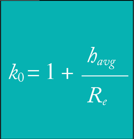
To use this map projection system for a project and to place the map projection surface near the ground, we conventionally define the scale factor as shown in the equation below where havg is the average height of the project typically and Re is the radius of the Earth. The mean radius of the Earth is typically used in these computations, which is 6,371,000 m or about 20,902,000 ft.
 When designing a low-distortion projection, the grid origin is placed near the center of the southern edge of the project extents. This minimizes the difference between the geodetic and grid azimuths for the project caused by the convergence angle. However, it will not eliminate these differences, so the difference between the grid and geodetic azimuths must be taken into account no matter whether you are using a low-distortion projection or state plane coordinates. Finally, the false northing and easting can be selected to prevent having negative coordinates in the current or future projects.
A low-distortion projection for Luzerne County, Pennsylvania is created to demonstrate this process. The WGS84 ellipsoid is used, which has a semi-minor axis (a) of 6,378,137 m and a flattening factor (f) of 1/298.257223563. The dimensions of the county are nearly square with sides approximately 200 km in length. Thus, the transverse Mercator map projection was chosen for the low-distortion projection.
The county’s geographic boundaries are between (40°53’30” N, 76°19’30” W) and (41°26’00” N, 75°35’30” W). As was stated, the grid origin for the projection is typically placed near the middle of the southern border of the map projection. However a more uniform distribution distance precision is obtained by placing the grid origin (φ0, λ0) at the center of the county or at (41°09’45″N, 75°57’30″W). Note that when determining the defining parameters for this projection, it is wise to round values to the nearest second or even tens of seconds.
Since we do not wish to have negative coordinates and there should be some overlap into southern and western bordering counties, the false northing and easting (N0, E0) were selected as (120,000 m, 120,000 m). The county has an approximate variation in elevation between 500 ft to 2200 ft. Thus, it provides a variation in elevation that will be difficult to match over its extents, which will demonstrate the limitations in using low-distortion projections to cover regions with significant elevation variation. Common practice is to set the map projection surface at the average elevation of the project, which means an average elevation of 1350 ft or 411.481 m. The average geoid height for the county is about −32.4 m. This would mean an average geodetic height, h, of 379.1 m.
Scales change in an east-west direction for a transverse Mercator map projection. Thus, to test the precision of the projection, 1000-ft lines were computed using geodetic computations at each corner of the county and at the 500-ft and 2200-ft elevations. Low-distortion projection coordinates for the endpoints of these lines were then computed and grid distances derived from these coordinates. These grid distances were then compared to the ground distances using a precision.
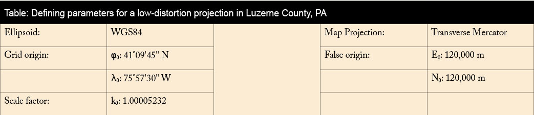
After a first attempt using the average elevation for the county to compute k0, it was found that the distance precisions at the upper and lower elevations varied significantly, and thus the design elevation was lowered to 1200 ft, or 375.76 m. This resulted in a geodetic height of 333.36 m for the design. Using the average radius of the Earth of 6,371,000 m and a design height for the mapping surface of 333.36, the defining scale factor k0 at 1200 ft is 1.00005232, which was determined using the equation stated previously.
These defining parameters for the low-distortion projection in Luzerne County are summarized in the table above. If the coordinates generated by the new low-distortion project are to have future use, these values must be documented and saved along with the defining ellipsoid.
Using the defining scale factor, which is greater than one, will raise the map projection surface to the elevation of 1200 ft in the county, thus minimizing the difference between the observed horizontal distance and its equivalent grid distance. Testing the low-distortion projection at its extremities provides the worst-case scenarios for distance distortion. In this case, the county-wide projection provided a distance precision in the worst case of 1:24,000. When distances are observed closer to the 1200-ft design elevation/orthometric height, the difference between the observed horizontal distance and the grid distance will approach 1:1. Of course, at 1200 ft, there will not be any difference between the observed horizontal distance and the grid distance.
While 1:24,000 precision may be adequate for many surveys, it is still below the precisions that can be achieved with today’s instruments. This distortion occurs because of the elevation variation in the county. However, better results can be obtained in regions where the variation is elevation is not quite as large as it is in Luzerne County. Still, even this low-distortion projection provides better distance precisions for the county than that available with state plane coordinates. However, it only covers an area of 907 sq. mi. rather than half of the state. As a comparison, using state plane coordinates and not properly reducing observed horizontal distances will result in distance precision for the observations at 2200 ft of only 1:6700.
The advantages of creating a low-distortion map projection for a large project are obvious. Once created, the difference between an EDM-observed horizontal distance and the reported grid distance from a GNSS survey can become minimal and often negligible. Distances computed from coordinates do not need to be converted from their map values during a construction layout project. Another advantage over state plane coordinates is that the false origin of the map projection can be placed near or in the project as done in this example, and thus the coordinates can be significantly smaller than what is typically encountered when using state plane coordinates.
Additionally, the projection can be designed to cover a relatively large region for large projects, such as an expansive multi-year project in a county. Also since the low-distortion map projection uses standard map projection formulas, it is possible to link the project to the National Spatial Reference System. This would not be true if arbitrary coordinates were created and a localization process was used to convert the GNSS observations into this arbitrary coordinate system. (See the December 2013 issue of Professional Surveyor on xyHt’s website.) Additionally, commercial software is available to create and use these independently created low-distortion map projections.
In Part 3 of this article, I explore the disadvantages of a low-distortion projection and propose another solution to the grid-versus-ground problem that still involves using the state plane coordinate system. To the surprise of some, this final approach is readily available, already built into software, easier to develop, and can provide much better distance precisions than the low-distortion projection developed in this article. Until then, happy surveying.