Single Project Factor

Here concludes a four-part series of articles about transformation of observations, spanning from September and December 2014 to March 2015. Part 1 covers how to transform surface observations into a geocentric coordinate system so that they can be compared to GNSS baseline vectors. Part 2 is about how the creation of a low-distortion map projection will bring the mapping surface up to the ground and thus provide a close comparison between GNSS and optical observations. Part 3 discusses some disadvantages in using a low-distortion projection.

This conclusion discusses an alternate method that can be easily implemented in the field with a survey controller, which is already available.

Single Project Factor Using State Plane Coordinates

A single project scale factor is determined as a single combined factor for the project. The requirement for this approach is that the distance distortion be better than those achievable using optical instruments, which in this case I will assume is 1:50,000. 

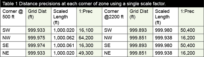
To demonstrate this I refer to my previous article on the low-distortion projection for Luzerne County, Pennsylvania. The 1983 PA-North zone scale factor at the center of the county is 0.99997777. The elevation factor at the average elevation of 1350 ft is 0.99993542. These two factors create a combined factor of 0.99991319.

Table 1 shows the distance precision at each corner of the region using the two extreme elevations. Note that lesser distance precisions are better than 1:16,000, which is worse than that produced by the low-distortion projection at 1:24,000.

However, it does show this precision at the extremes only, which is on the northern edge for the county. Again, in an area where elevation variations are not as large, the single combined factor will produce much better results.

Since a single project rarely covers an area of 907 sq. mi., it is often possible to use a single combined factor (which I will call a project factor from now on) that produces precisions that far exceed typical survey precisions. This project factor, which is an average combined factor, can easily be developed for much smaller regions. If this results in a precision that is better than the precision of the survey, state plane coordinates will be produced at the precision of the survey.

For example, assume that your project is limited to the City of Wilkes-Barre in Luzerne County where the elevations vary from about 500 ft to 900 ft. The city covers an area of 7.2 sq. mi. Using an average scale factor of 0.99996148 and an elevation factor of 0.99996699, which was computed for an elevation of 690 ft, the project factor for the City of Wilkes-Barre is 0.99992847.

If this value is entered into the survey controller as the project factor, the least precision achieved in the city would be 1:88,400 at 900 ft in the northeast corner of the city. However, a majority of the city has a distance precision over 1:100,000. Since these precisions are much better than the precision achieved by a typical optical survey, the resulting coordinates produced by this survey will represent state plane coordinates at the accuracy of the survey.

Survey controllers have the capability of applying a single factor in a project built into the software. It is typically defined at the creation of the project. This value typically defaults to 1. However, if the value were changed to 0.99992847, the controller will shorten all observed horizontal distance by this value to compute the state plane coordinates in the City of Wilkes-Barre. When staking out points, it will divide the grid distance determined by inversing state plane coordinates by this factor to determine the appropriate ground length.

In essence, whether running a traverse or performing a stakeout, the controller will handle the grid-versus-ground problem using the project factor at a precision of 1:88,000 or better. Furthermore, nothing, not even the project factor, needs to be saved for later use since the coordinates derived from the survey would be state plane coordinates at the accuracy of the survey.

Since it is actually less time-consuming and less difficult to determine the project factor for a survey than to create and check a low-distortion projection for its accuracy, this process is much simpler to perform. Additionally, since the resultant survey coordinates are state plane coordinates, the aforementioned problem associated with using a low-distortion projection is avoided.

Thus, there would be no need to maintain defining parameters or the project factor since state plane coordinates are being generated by the survey at the precision of the survey. If another project required you to revisit the control established by the first survey, the coordinates are still state plane coordinates.

Controller Software

Using total stations, we collect observations in three dimensions but then work in either two or one dimension. Using the capabilities of a total station, it is possible to develop controller software that properly reduces each distance to the SPCS mapping surface.

This would require an approximate elevation for the initial control station to be known. I say “approximate” since a code-based elevation for the total station would be adequate to provide a sufficiently accurate elevation factor, which could be used in the reduction of observed horizontal distances.

Using this approximate elevation and the three-dimensional capabilities of the total station, approximate elevations could be determined for any point surveyed. Thus, the survey controller software could properly reduce individual distance observations to the mapping surface based on its average elevation.

Additionally, the controller could also bring the grid distances back to the surface when performing stakeout based on its endpoint elevations. Thus we would not be talking about distance precisions since a map projection system provides a 1-to-1 relationship between points on the surface of the Earth and the map projection. This process would work at any elevation and any location in the country, removing the responsibility of properly working map projections from the surveyor. Thus, we wouldn’t even need to think about creating a low-distortion projection.

It is possible that some software vendors have developed such software, but I am not aware of any. However, previous experience shows that if surveyors ask for such capabilities, the vendors will produce the software. An example of this is the multitude of low-distortion projections that were created in Wisconsin at the county level. These now appear in my GNSS software even though I have no need for them in Pennsylvania.

For those of you wanting to minimize the problems with map projections, ask the vendors to develop this software to relieve you of the reductions. However, be concerned: this is leading the profession more and more into a trade status since it is a situation where software is developed to alleviate the professional of the responsibility of knowing how to do it. Just another problem to be concerned about.

Conclusions on Low-distortion Projections

I believe that companies are taking on more than they realize when using low-distortion projections simply to avoid the difference between the grid distance between two points versus its horizontal length on the ground. As discussed here and in the first article in this series, a single combined factor for a project can be entered into your survey controller. The controller will automatically reduce observed horizontal distances to map distances when computing coordinates and reverse this procedure so that ground distances are used when laying out a project.

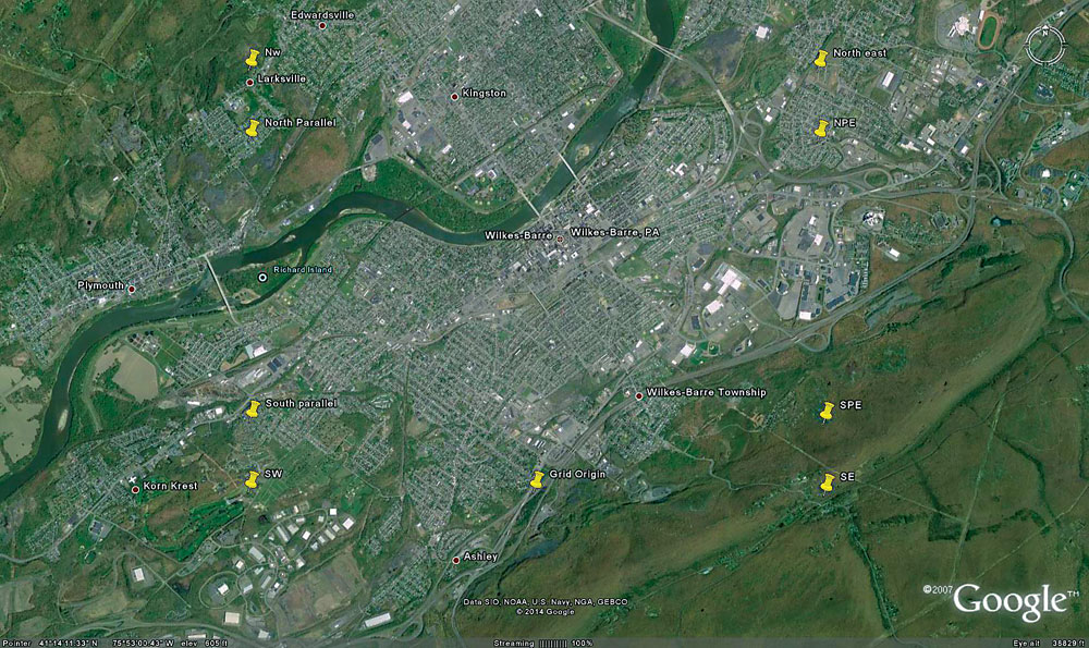
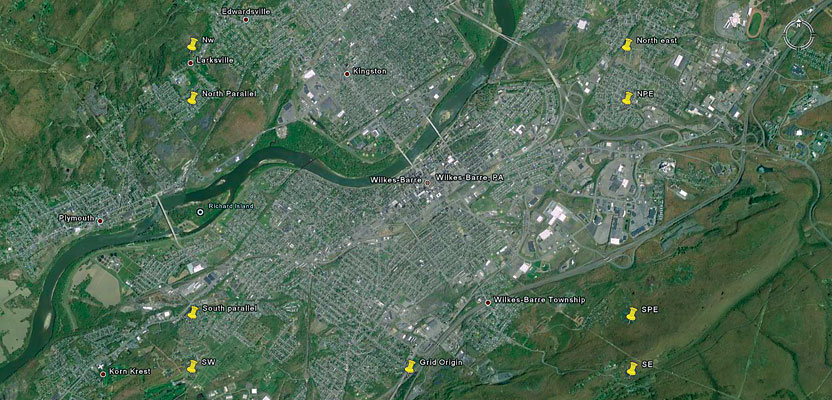
This Google Earth view of Wilkes-Barre, Pennsylvania, shows marks for the corners and standard parallels for the low-distortion projection.

Additionally, proper use of state plane coordinates will automatically put the project in the National Spatial Reference System (NSRS). With NGS software such as OPUS, it is easy to put any project on the NSRS with a GNSS receiver.

While personal, low-distortion projections may appear to be the solution to the grid-versus-ground problem, they can create their own problems in the future. Finally it is possible at this point to contact the NGS and have your future map projection surface placed closer to the Earth’s surface in future state plane coordinate systems, which would create nationally maintained low-distortion projections. Due to the areas covered by the state plane zones, it will never exactly match the ground observed horizontal distances, but it can be designed to be much closer to the surface than they are presently, thus reducing these differences. (I discussed this possibility in a June 2013 issue of Professional Surveyor).

In this series of articles, I demonstrated how conventional instrument observations could be transformed into changes in geocentric coordinates, how a low-distortion map projection could be used to bring the mapping surface up to the measurement surface, and the advantages and disadvantages in this approach, and I demonstrated how to compute and implement a project factor for a survey. It is your choice which method to use since all could be used to provide the ground distances.

I personally chose a single project factor because it is easy to compute and implement. I can use it in small projects or large projects with equal success. It means I am working in the NSRS and does not require that I maintain defining map projection parameters for future use or for transformation into the NSRS.

Hopefully these articles have helped you understand the problem and potential solutions. Until next time, happy surveying.