In this article, I demonstrate the proper computations used when working with conventional surveys that use state plane coordinates. I purposefully selected a traverse in Pennsylvania that climbs about 1100 ft in its 2-mi length. By examining this particular site as an example, the reader can see the effects of elevation on the computations and the traverse closure errors. Finally, I present simpler methods that can be used when elevation differences in the traverse are not as great.

An Example Traverse

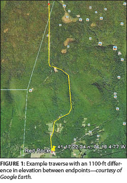Figure 1 depicts the path of a traverse that runs primarily South to North in the Zone 3701 of the Pennsylvania State Plane Coordinate System 1983 (SPCS 83). This traverse follows a road that runs from the intersection of two state highways and terminates near the entrance of a state park. It also climbs a hill that varies in elevation by about 1100 ft from the beginning to its terminus. 



The purpose of demonstrating the computations for this traverse are two-fold. First, it demonstrates the methods used to properly reduce the observed distances to their equivalent grid lengths. Second, it demonstrates the importance of reducing distances using both the scale factors and elevation factors. The traverse is approximately 2.25 mi long (10,951 ft between endpoints), yielding an average grade of about 9.9% over its entire length.



The observations for this link traverse are shown in Table 1. The approximate elevation (H) at each station was obtained from a map. These approximate values are sufficient to determine an approximate elevation factor for later distance reductions. The geoid height (N) was obtained using approximate coordinates (discussed later) and the National Geodetic Survey (NGS) Geoid 12A model (www.ngs.noaa.gov/GEOID/GEOID12A/). The approximate geodetic height in meters for the stations was derived usingEquation (1). The angle at the Station 2 was to an azimuth mark, which had a geodetic azimuth of 171°10’29.6″. The horizontal distances were recorded in units of feet. 



The SPCS 83 NE coordinates of the Station 2 in feet are (413892.42, 2,366,343.66) and for Station 12 are (423,389.71, 2,366,191.75). The geodetic azimuth to the last azimuth mark of the traverse is 359°19’11”. 



Using the NGS Geodetic Toolkit software (www.ngs.noaa.gov/cgi-bin/spc_getgp.prl) and converting the station coordinates to meters, we see that the convergence angle at the Station 2 is 0°57’28.13″, and its scale factor is 0.9999592. Inversing the coordinates at Station 12 on the same web page, we find the convergence angle at this station to be 0°57’28.19″ with a scale factor of 0.9999583. From the initial 57’28” convergence angle combined with the fact that the terminal stations are 10,951 ft apart, we can see that if no correction to the geodetic azimuths were made, all the station coordinates would be rotated and the final computed station coordinates would disagree with the given coordinates by more than 183 ft at Station 12. 



Thus, to start the computations we must first convert our geodetic azimuths to grid azimuths using Equation (2)where Az is the grid azimuth of the line, α the geodetic azimuth of the line, and γ the convergence angle at the station with a longitude of λ, which is derived in a Lambert Conformal Conic mapping zone by Equation (3)where λCM is the positive western longitude of the central meridian, which is 77°45′ W in Zone 3701, and n (also known as the sin φ0) is a derived zone constant, which is 0.661539733812. From Equation (2) we see that the grid azimuth to the first azimuth mark is 171°10’29.6″ − 0°57’28.13″, which is 170°13’01.5″. Similarly, the grid azimuth from the last station to its azimuth mark is 359°19’11” − 0°57’28.19″, or 358°21’42.8″.



From the difference in the scale factors at the two endpoints, we see that there are five common digits (0.99995) and one that varies, yielding six significant figures in the scale factors. Because our longest observed distance contains only six digits, this implies that we may be able to get by with a single scale factor to reduce our observed horizontal distances. However, this assumption would be incorrect because the elevation differences of nearly 1100 ft over the entire length of the traverse yield elevation factors that vary significantly in the fifth decimal place. 



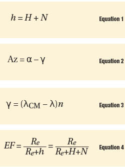For example, at the first station with an approximate geodetic height of 1165 ft (355.225 m), we find the elevation factor (EF) is 0.99994425 from Equation (4)where Re is the average radius of the Earth, which is 6,371,000 m. At Station 12 with an approximate geodetic height of 684.761 m, the elevation factor is 0.99989253. Notice that at Station 12 the elevation factor yields a distance precision of only 1:9300 regardless of the scale factor.



At this point we are almost ready to perform standard plane traverse computations. We have our starting and ending azimuths in the PA North zone map projection system along with the initial and closing coordinates. However, the distances must still be reduced to the map projection surface. 



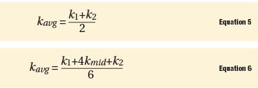
As shown in Figure 2, this reduction takes two steps. First, the observed horizontal distance (Lm) must be reduced to its geodetic equivalent (Le). This is done using the average elevation factor for each traverse course. The second reduction involves taking the geodetic length of the line and reducing it to map projection surface (Lg). This reduction is done using a function of the scale factors on each course. 



For typical surveying work where the length of the lines are relatively short (as shown in this example), an average scale factor using the two endpoints of the lines may be used with Equation (5) where k1 and k2 are the scale factors of the stations at the ends of the line. 



However, for longer distances, a weighted average of the scale factors should be based on Equation (6) where kmid is the scale factor at the midpoint of the line. The typical distances observed by surveyors rarely warrants using Equation (6). The deciding factor will be the number of common digits in k1 and k2 as compared to the length of the lines. 



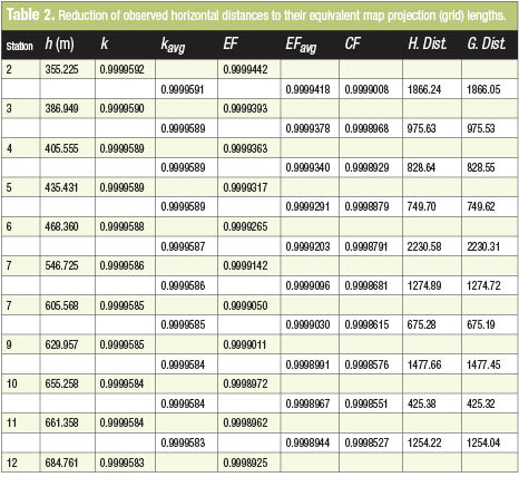
For example, if a distance could be observed between Stations 2 and 12 then, as previously mentioned, the scale factors vary in the sixth decimal place (0.9999592 and 0.9999583). Because the overall distance between these two stations is about 10,951.00 ft, which has seven digits, it would be wise to use Equation (6). However, in this example our longest observed horizontal distance is 2230.58 ft, so we can reasonably assume that Equation (5) is sufficient. As can be seen in Table 2, the scale factors at the endpoints of each line never vary before the seventh decimal place, which justifies using Equation (5) instead of Equation (6) because our distances only have six digits at most. 



To create Table 2, we need to know approximate elevations at the endpoints of each distance. These were obtained from a map sheet. To obtain the scale factors (k), approximate station coordinates are also needed, as was previously mentioned, to obtain geoid heights at each station. They are computed using standard traverse computations with observed horizontal distances and grid azimuths. 



These approximate station coordinates are then used to determine the scale factor and geoid height at each station using appropriate software, such as that provided by the NGS. These values are shown in the column headed by k in Table 2. The elevation factor at each station is obtained using Equation (4) and an average radius of the Earth. Because these scale factors are unitless, the distances can have any units. However, it is important to remember when computing Equation (4) to have Re, h, H, and N in the same units, which is why I chose to convert my station elevations to meters.



Once the scale factor (k) and elevation factor (EF) are determined for each station, they are averaged. Another approach is to average the geodetic heights of the endpoints to obtain the average elevation factor directly from Equation (4). 



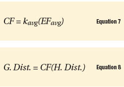The combined factor (CF) for each course is then computed as Equation (7). This combined factor is multiplied by the respective observed horizontal distance to obtain the equivalent map projection (grid) distance, or Equation (8).



Using grid azimuths and grid distances, the traverse is computed using standard plane computational techniques. If the traverse in this example had been computed using the observed horizontal distances and grid azimuths, the traverse misclosure would be 1.25 ft with a relative precision of 1:9400. However, using the grid distances, the linear misclosure of the traverse is 0.32 ft with a relative precision better than 1:36,000.

The Problem with Ground Coordinates

Even though there is no recognized coordinates system on the surface of the Earth, some surveyors insist on trying to perform state plane coordinate computations on the ground. These surveyors realize that if they simply divide the state plane coordinates at each station by the combined factor for the station, they can obtain ground coordinates. While this much is true, caution must be taken when using ground coordinates in any computations or layout situations. The reason for this is the elevation of the stations. 



Using the preceding example, we have a combined factor at Station 2 of 0.99990340. If this is divided into the given northing and easting coordinates for Station 2, we obtain NE ground coordinates of (413,932.405, 2,366,572.265). At station 12, we have a combined factor of 0.99985080, which when divided into the coordinates for Station 12 yields NE ground coordinates of (423,452.887, 2,366,544.828). 



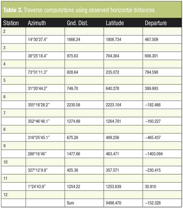Using the observed horizontal distances, Table 3 shows the initial traverse computations. The difference in the ground coordinates of Stations 2 and 12 are 9520.482 in latitude and -27.438 in departure. As can be seen in Table 3, these values differ from the sum of the latitudes and departures computed with observed horizontal distances by -22.012 ft and -124.891 ft, resulting in a linear misclosure of 126.382 ft and a relative precision for the traverse of 1:100.



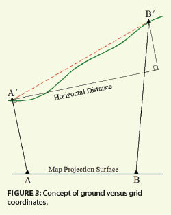
The reason for these large discrepancies is due to the difference in elevation between stations, which is why this particular traverse was chosen. As can be seen inFigure 3, the grid coordinates lie on a plane surface. However, the ground coordinates are projected radially from the center of the Earth through their grid locations to the topographic surface of the Earth. Thus, the horizontal distance does not project to the second station correctly because the horizontal plane at any station is not parallel with the map projection surface. This difference is seen in the computational example. This error will also occur during layout. Thus, it is not prudent to use ground coordinates to lay out alignments or structures. They simply do not match the theory of map projections. 



Now, some may state that they did not see any unreasonable error when using ground coordinates. This may be true if the area of the survey is reasonably flat. In this case the difference in elevations between stations is small and, similarly, the error caused by using ground coordinates may be small. But this is living very dangerously and could not be supported in a court of law if an error does occur.

The Project Combined Factor Method

The computations shown in this article are not complicated, but they certainly do require more effort than simply using the observed horizontal distance. If only the Earth were flat rather than round, this would not be a problem. Well, it is not, so we have a choice. We can use geodetic computations when laying out or observing a station, or we can use a map projection and pretend the Earth is flat. The latter will provide the same results as geodetic computations but requires that all observations are on the map projection surface. 



To simplify the computations, manufacturers have developed routines in their survey controllers to handle map projection surfaces. In fact, one obvious method is displayed each time a project is started. Part of the settings for a project is a scale factor. When using state plane coordinates, this scale factor should be set to an average combined factor for the project. 



Using the combined factors for Stations 2 and 12, we see that the average combined factor is 0.99987712. If the observed horizontal distances are all reduced using this average combined factor, the traverse misclosure would be 0.40 ft for a survey relative precision of 1:29,000. This differs from the correct computations by only a 0.08-ft difference in the 11,758-ft traverse. 



The reader should remember that this survey was selected to demonstrate the proper procedures in reducing observations to a map projection surface. In typical surveys, this large of a difference is seldom seen. In fact, it is more common to see differences only in the 0.001 ft between a single combined factor and proper methods. However, even with that said, it is only 0.08 ft in 11,758 ft or 1:147,000. It is up to the professional to decide if this difference is acceptable for the purpose of the survey.



During layout, the survey controllers will use the single scale factor to determine the proper ground distance. To do this it inverses the map projection coordinates to determine the distance on the map projection surface between the two stations. It then uses a rearranged Equation (7) and the project scale factor to determine the horizontal length at the surface between the two layout stations. Simply put, today’s survey controllers can handle map projection computations both in the direct and inverse modes when a proper combined factor is supplied for the project, thereby removing the drudgery of doing these computations by hand and simplifying the survey.



The bottom line is that only map values should be used to compute mapping coordinates if you wish to compute state plane coordinates and maintain the accuracy of your survey. However, as was shown in this article, it is possible to minimize this work if a single combined factor can be used in distance reductions. When this is the case, a project scale factor is determined for the survey and entered into your survey controller project. The software will then correctly perform the computations whether it is an observation or stake-out situation. This project factor should be part of the metadata of the survey and retained for future reference, just as the original observations are retained.



In areas where geographic information systems (GIS) are being implemented, the state plane coordinate system provides a common reference plane, which allows surveys of various types to be combined into a cohesive map. However, if observations are not properly handled in the computations of the coordinates, the result will be a mismatch of mapping elements that are located by various surveys and, in the end, a map of little or no value.