In previous articles, I discuss two rudimentary techniques that can be used to identify blunders in data.
However, anyone who has used an advanced least squares adjustment package knows that such software often uses a post-adjustment statistic known as the tau criterion. The tau criterion is a modification of a method known as data snooping, which was introduced by Willem Baarda in the mid-‘60s.
In this article, I discuss these two post-adjustment blunder detection techniques. While the math in this article may not be for all to enjoy, the post-adjustment procedures—that should be followed when possible observational blunders are uncovered using either data snooping or the tau criterion—are important for all users to understand.
Data Snooping
In the previous article (November 2016), I applied the critical value from the t distribution to the estimated error of the observation to identify residuals that were larger than estimated, and thus to identify blunders. This technique can be referred to as a crude but effective method.
A more refined procedure is not as dependent on the estimated error for the observation but rather computes the uncertainty in the residual of the observation. As previously noted, Willem Baarda presented this method in a series of papers in the mid- to late-1960s using geodetic data.
The method, called data snooping, presented more than just a method of identifying blunders in geodetic data. Its theoretical background is based in error propagation and a principle known as the general law of the propagation of variances. This law states that when working with a set of functions, the errors in the observations will propagate through those functions as shown in Equation (1).
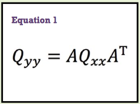
In Equation (1):
• Qyy is the cofactor matrix of the resulting
function from which the variance-co variance matrix for the function can be computed,
• J the coefficient matrix of the observations,
• J T its transpose (Ghilani, 2016) and
• Qxx the variance-covariance matrix of the
unknowns, which the least squares adjustment provides as part of the solution for the unknowns.
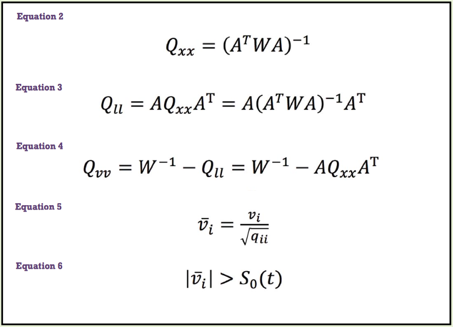
The computation of Qxx is shown in Equation (2). Here, W is the weights of the observations prior to the adjustment (Ghilani, 2016a and 2016b).
To propagate the errors in the unknowns from Qxx to the adjusted observations, we must apply Equation (1) to arrive at the cofactor matrix for the adjusted observations, Qll, as shown in Equation (3).
Finally the cofactor matrix in the residuals, Qvv, is computed as shown in Equation (4).
If all of this is confusing, it can be stated simply that the errors in the observations have been propagated from the original observations, to the unknown parameters, then to the adjusted observations, and finally to their residuals v. The actual statistics and mathematics can be left to the mathematicians, statisticians, and programmers.
What is important in these four sets of equations is that the errors in the original observations have been propagated to the residuals so that we can now determine the a posteriori (after the adjustment) standard deviations of the residuals. If you are asking, “Why compute standard deviations for the residuals?” it is because now we can estimate how large a residual is unacceptable for any given observation at any level of confidence/probability.
In his derivation, Baarda assumed that there was only one blunder in any set of data. If this were the case, then the size of the residual in that observation would be directly related to the standard deviation in the residual. The standardized residual is then computed as shown in Equation (5), where:
• v–i isthestandardizedresidualofan observation,
• vi the residual of the observation, and
• qii the diagonal element of the Qvv matrix
that corresponds to the residual, vi. Again the mathematics here is not important. However, you now know what the standardized residual column represents in the output from your commercial least squares package.
Baarda used a single critical value from the t distribution to decide if an observation with standardized residual v–i is in fact a blunder. Mathematically speaking, an observation is identified as a possible blunder if its absolute value is greater than S0 (t), as shown in Equation (6).
In Equation (6), S0 is the standard deviation of unit weight for the adjustment; that is, the square root of S02 (Ghilani, 2015), and t is from Student’s t distribution, which Baarda originally suggested to be 4.
The proper use of the method is to remove only one observation from the data set and then rerun the adjustment.
However, the application of this process in photogrammetry suggested that a critical t value of 3.29 worked well in identifying blunders in data. This value has been used ever since when this method is applied in most instances. This process is similar to the method I suggested earlier, although in this case the critical t distribution value is always assumed to be a specific value assigned by the user.
One caveat on this process is that Baarda assumed that the data set had only one blunder. Since this is not the case necessarily, the proper use of the method is to remove only one observation from the data set (that is, the one with the largest standardized residual) and then rerun the adjustment. This process of removing one observation at a time is continued until the user does not find any observation that satisfies Equation (6). At this point the data is assumed to be clean from blunders.
Now the user needs to reinsert each observation that was detected as a blunder back into the adjustment to see if it is again detected as a blunder. Recognize that other blunders could have caused a large residual on a particular observation, which resulted in its incorrect removal from the data.
Anyway, at this point the basic premise that the data set contains one blunder is satisfied because the only detectable blunder left in the set of data is the one being reinserted. If the observation again satisfies Equation (6), the observation is statistically identified as a blunder or outlier and needs to be discarded or re-observed.
While this process may seem laborious, it really isn’t because the typical adjustments can be performed in less than a second. Additionally, the process can be automated in the software. Using a critical t value of 3.29 yields data that is clean from blunders at about a 99.9% level of probability. I often use the statement that the data is Ivory soap clean of blunders.
The tau Criterion
In the middle of the 1970s, Alan Pope, a statistician with the National Geodetic Survey, identified a flaw in the data snooping method, which can be seen in Equation (6).
Recall that the standard deviation of unit weight S0 is computed as shown in Equation (7). (The terms in Equation (7) have been previously defined.) What Pope realized is that S0 was tainted by the observation with the detected blunder and thus had a large residual vi. Thus, S0 was not a good estimate of σ0 for the adjustment.
He suggested that a better critical value to use when rejecting observations as blunders was from the tau (τ) distribution. The critical value for the tau criterion is based on the t distribution, and can be computed as shown in Equation (8), where r is the number of redundant observations in the adjustment and t is the critical t distribution value with r – 1 degrees of freedom and α level of confidence.
It is hard to believe now, a mere 40 years later, that he then developed tables for varying the number of redundant observations and α levels due to the complexity of computing Equation (8). In today’s world, a spreadsheet can compute this equation as well as most software packages.
It should also be pointed out that α has to be transformed for the number of nonspur observations for what he referred to as a transformation for control of the Type I error.
The only difference between his suggested method and that proposed originally by Baarda is the τ critical value is used to determine if an observation is identifiable as a blunder rather than a t statistic critical value. The remaining procedure—of removing only one observation that is detected
as a blunder at a time and then reinserting these observations after the set of data is determined to be clean—did not change.
Often software that has the tau criterion built into it will highlight or mark observations that are statistically detected as blunders. Some software will automatically go through the process of removing these observations. No matter the method, these procedures do an excellent job of removing blunders from data sets when the observations are correctly weighted (Ghilani, 2013a).
This is a key for all of these statistical blunder detection methods. That is, the weights of the observations must be correct. Correct weighting of conventional observations was discussed in the previously cited article.
While much of what is presented here seems to be complicated, those of you who use a commercial least squares package to adjust your data now have a feeling on how to identify and remove blunders from a set of data. When performed correctly, either of these methods works exceedingly well. I programmed these procedures back in the 1980s and have used them over and over again to identify possible blunders in the observations.
Often these blunders uncover incorrect field procedures or computational methods that can hopefully be avoided in the future if the creator is made aware of what went wrong.
It is important when uncovering blunders to identify what happened to create the blunder in the first place. Often these blunders uncover incorrect field procedures or computational methods that can hopefully be avoided in the future if the creator is made aware of what went wrong.
Like the distance that students repeatedly measured incorrectly, once identified it was important for me to correct the mistake so that the students would hopefully remember never to do it again in their professional lives.
For those of you wishing to see the mathematical development of these and other equations I have presented in this series of articles, I refer you to my book, Adjustment Computations. (Ghilani, 2010).
In the next article I look at the computation of error ellipses and other statistical quantities. Until then, happy surveying.
References
Ghilani, Charles D. 2010. Adjustment Computations: Spatial Data Analysis. John Wiley & Sons, Inc. Hoboken, NJ.
–––––. 2015. “Sampling Statistics: The t Distribution.” XYHT accessed here
–––––. 2016a. “A Correctly Weighted Least Squares Adjustment, Part 1.” XYHT accessed here
–––––. 2016b. “A Correctly Weighted Least Squares Adjustment, Part 2.” XYHT accessed here
–––––. 2016. “What is a Least Squares Adjustment Anyway?” XYHT, accessed here.