Standard Error Rectangle and Error Ellipse

Figure 1: The standard error rectangle and error ellipse.or ALTA/NSPS Land Title Surveys.

What is an error ellipse? One of the advantages of a least-squares adjustment over other methods is that a byproduct of the adjustment is not only the most probable values for the unknown coordinates but also standard deviations on these values

Suppose for a moment that we are computing the coordinates of station B shown in Figure 1 using an azimuth AZ_AB with an uncertainty of S_Az and a distance AB with an uncertainty of SD ft. Even if we consider the coordinates of station A to be perfect, the coordinates of B will have uncertainties of S_x and S_y due to the errors in the azimuth and distance.

This uncertainty in the coordinates for the position of B results in a standard error rectangle that surrounds B. This rectangle represents the area that the true coordinates of station B will be about 68% of the time. It will have dimensions of 2S_x by 2S_y.

However, the standard error rectangle does not depict the actual error in the coordinates. This is where an error ellipse comes in. As shown in Figure 1, the standard error ellipse is bounded by the standard error rectangle. It is the results of the bivariate (x and y variables) distribution shown in Figure 2(a).

If Figure 2(a) is contoured, Figure 2(b) is the results. Figure 2(b) depicts error ellipses at various levels of probability.

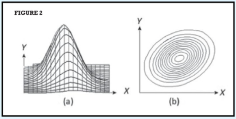
Figure 2: (a) A wire diagram of a bivariate distribution and (b) the isogonic lines of a contour plot of (a).

As can be seen in Figure 1, the bivariate distribution does not completely fill the standard error rectangle, but it does show the bounds of the true coordinate values at a specific probability level for station B given the uncertainty in both the azimuth and length of line AB. The larger the error ellipse, the more likely it contains the true coordinates for station B.

In essence, we know that the coordinates contain error. Thus, what the 2016 ALTA/NSPS survey standards are stating is that you must be within 0.07 ft of the true coordinates of a station 95% of the time. This means that 95% of the time a competent surveyor can come within 0.07 ft in a subsequent resurvey.

Quite honestly, the standards also allow for an additional 50 ppm for the distance between the two stations being tested. However, this would add only an additional 0.004 ft for a 500-ft distance between stations or 0.016 ft for a 1000-ft distance. In essence, it does not significantly increase the allowable error for typical distances encountered in most surveying practice.

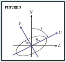
Figure 3: Components of the standard error ellipse.

Computation of Error Ellipses

The components of the error ellipse are shown in Figure 3. The t angle is the amount of rotation that is required to make the correlation between the (n, e) pair of coordinates equal to zero. It is measured from the positive N axis.

The major axis of the ellipse is the U axis and the minor is the V axis. The length of the semimajor of the ellipse is given by S_u which corresponds to the largest error component at the station, and the length of the semiminor axis of the ellipse is given by S_v which is the smallest error at station.

One of the advantages of a least-squares adjustment is that it has a statistical basis. Thus, at the end of the adjustment, uncertainties in the coordinates can be computed, which are the standard deviations in the northing and easting coordinates.

However, as was previously stated, these uncertainties are not in the direction of the largest error at the station typically. They are also correlated. Correlation means that as one coordinate at a station changes, the other must also change.

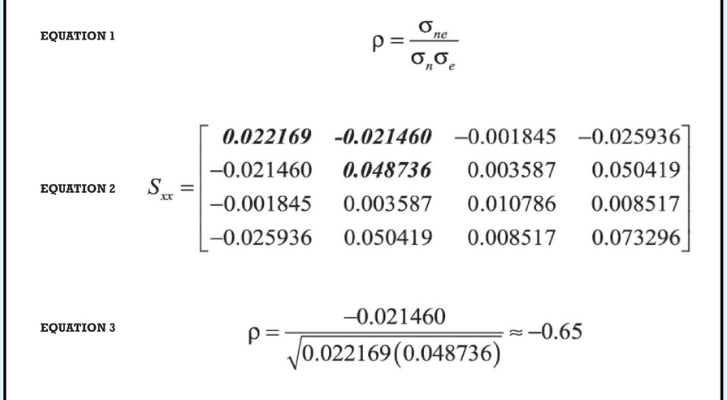
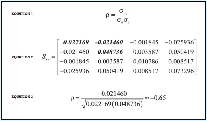
This can be seen in Figure 1, where if we change the value of the northing for station B, the value of the easting must also change to maintain the azimuth of AB. This link between the coordinate values can be mathematically expressed by the Pearson correlation coefficient, which is defined as in Equation (1) where σ_n is the standard deviation in the northing, σ_e the standard deviation in the easting, and σ_ne the covariance between the two unknowns.

Foundations for Computing Error Ellipses, figure 2

For example, assume we have the covariance matrix, S_xx shown in Equation (2) from an adjustment of a horizontal survey involving only two stations with unknown coordinates. (As an aside, the covariance matrix is the inverse of the normal matrix we used to simultaneously solve for the unknown coordinates.)

The survey had only two stations with unknown (n, e) coordinates. Highlighted in bold font is the variance in northing of 0.022169, covariance in the two unknowns of −0.021460, and variance in easting of 0.048736. The square roots of the variances for each of these diagonal elements, which are ±0.149 and ±0.221, would yield the northing and easting standard deviations for the station coordinates. We see that these elements are correlated since the immediate off-diagonal is not equal to zero with a value of −0.021460. This number indicates that as the northing of the station changes so must the easting.

By Equation (1) the correlation coefficient for the unknowns is as Equation (3). The correlation coefficient is always between −1 and +1. If it is negative, one unknown will decrease as the other increases. If they are positive, both unknowns will increase or decrease simultaneously. The closer to zero the coefficient is, the less correlation exists between the two unknowns.

As can be seen from Equation (3), the two unknowns are negatively correlated, meaning that as the northing increases the easting must decrease, or vice-versa. The correlation coefficient for the error ellipse shown in Figure 1 would be positive since the easting must increase as the northing increases to maintain the azimuth of the line.

Thus, in concept, the method to compute the semimajor and semiminor axes of the standard error ellipse is to rotate the 2-by-2 diagonal submatrix for each station by an amount that removes the correlation between the two components. In essence, we will be rotating the NE axis system to UV where there is no correlation between the U and V components. For those readers who are mathematicians, the process involves an orthogonalization on each 2-by-2 submatrix of the covariance matrix.

In the next article I demonstrate the process and discuss how we can increase the probability of the standard error ellipse to 95%. Until then, happy surveying.

Reference

National Society of Professional Surveyors, 2016 Minimum Standard Detail Requirements for ALTA/NSPS Land Title Surveys