Estimating Standard Errors in Angular Observations
In the previous articles (January and February 2016) I discuss the unreliability of standard deviations when they are computed from a small sample of observations, as well as how to estimate errors in centering an instrument over a well-defined point and how to estimate the standard error for electronically measured distances.
Here I look at the more complicated problem of estimating standard errors in angular observations.
The uncertainty in an observed angle is a function of several smaller errors, but first we need to understand the method that manufacturers use to classify their digital theodolites and total stations.
When the first digital theodolites were created, they realized that the user could no longer distinguish between the qualities of the instruments by viewing the circles through their reading scopes. (Sorry young’uns, this is way before your time.) Thus, the German manufacturers came up with the DIN18723 standard for digital theodolites.
All manufacturers then began to provide a DIN18723 standard for each instrument they sold, which indicated the instrument’s ability to point and read a single direction. Since then, the International Organization for Standards has published the ISO 17123-3 standard, which accomplishes this same function.
It is important to understand that these standards were created to provide a means of differentiating between the qualities of the instruments and are not a true measure of one’s ability to turn an angle with the instrument. However, it does show that different instruments will provide angles of different precisions.
Besides this, experienced surveyors realize that longer sight distances result in better angle observations. Additionally, surveying on property where large altitude angles are present results in larger angular misclosure errors, typically. Thus, not all angles observed have equal precision. So let’s look at each error individually.
First Angles
These consist of two-directional observations of the horizontal circles. Additionally, different surveying firms observe angles using a different number of sets. Most common among these are one (1DR) and two (2DR) sets of angles, which result in an average for the angle observation.
Note that if you are turning an angle only 1D then you are not compensating for the systematic errors present in your instrument. This may be acceptable in mapping and construction surveys, but it is not an acceptable practice in boundary or many other types of surveys.
Horizontal Angles
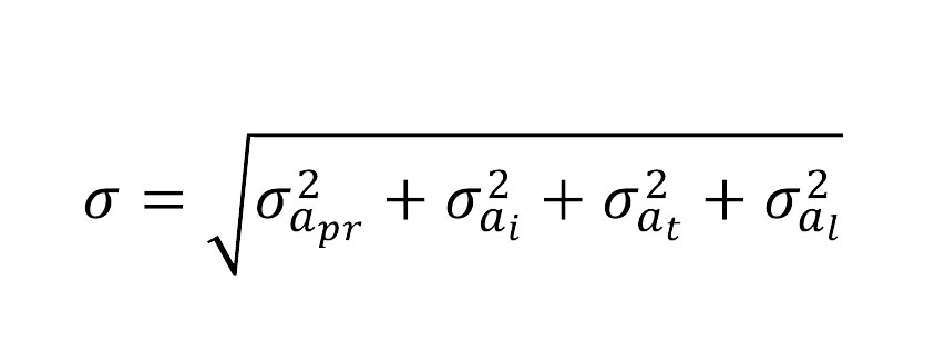
Equation 1
The major sources of errors in a horizontal angle consist of the quality of the instrument, which is:
- the pointing and reading errors, σαpr,
- number of times the angle is observed, n,
- the centering error of the instrument and target over their stations, σα1 , σαt ,
- and the leveling error of the instrument, σα1.
Each of these error sources contribute to the overall error in an observed angle. Because these error sources are independent of each other, the overall error in an angle observation using error propagation is shown in Equation 1.
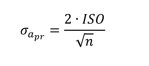
Equation 2
As previously stated, the standards are based on the observation of a single direction in both faces. As we repeat our measurements, this compensating error is also repeated for each pointing. The contribution of this error to the overall uncertainty in the angle is shown in Equation 2 where n is the number of times an angle is repeated and ISO the ISO standard for the instrument.
Now, if some of you are saying, “Wait, didn’t you just say that the ISO standard was not a true measure of an individual’s ability to turn and angle with the instrument?” the answer would be yes, but apart from determining each individual’s personal ISO standard with a particular instrument, this is the best estimate we have for the instrument.
It should be pointed out that I had our second-year students determine their personal ISO and have noted over time that some will be slightly better than the standard of the instrument, some will match the standard, and some will be slightly worse than the standard published for their instrument. In fact, the ISO standard matches their observational abilities and is thus a valid value for their personal abilities, statistically speaking. Thus, the DIN or ISO standards are a good estimate for this error contribution.
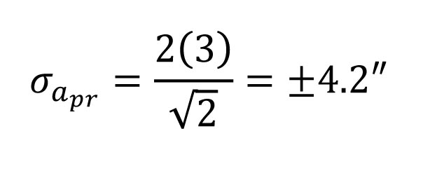
Equation 3
So, if an angle is measured 1DR (n = 2) with a 3” total station, the resulting contribution to the overall angular error is as shown in Equation 3.
This same angle observed 2DR (n = 4) has an error due to pointing and reading of ±3”, observed 3DR (n = 6) has an error of ±2.4”, and observed 4DR (n = 8) has an error of ±2.1”. It is interesting to note that the increase in angular precision begins to level off after eight repetitions or 4DR.
The target miscentering error is a function of the length of the sights. It is computed as in Equation 4 where:
- DBS is the length of the backsight,
- DFS the length of the foresight,
- σt the estimated error in centering of the targets, and
- ρthe conversion from radian units to seconds, which is 206264.8”.
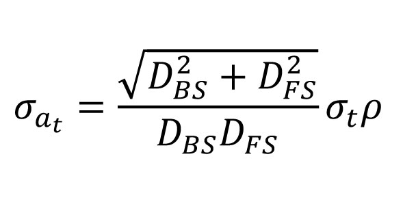
Equation 4
For an angle with both sight distances being 100 ft, the amount of error contributed to the angle with a target miscentering of only ±0.005 ft is ±14.6”. If both sight distances are 200 ft, it is ±7.3”; for sight distances of 400 ft it is ±3.6”.
From this we can see that short sight distances result in larger overall errors in the angles even though the miscentering error is the same. That is: in terms of the point’s coordinates, shorter sight distances have little effect on the coordinates of the stations but larger effects on the standard errors for the angles, which means that angles observed with short sight distances are subject to more error and should be weighted as such.
Similarly, the instrument miscentering error can be significant when the sight distances are short. The equation to determine its contribution to the overall angular uncertainty is shown in Equation 5 where:
- D3 is the length of the distance connecting the backsight and foresight stations, which can be computed using the law of cosines, σi,
- the estimated error in instrument miscentering, and
- other terms as previously defined.
Equation 5
This error is interesting because it also depends on the size of the angle, which affects D3. Again, assuming an instrument miscentering error of ±0.005 ft with a 90° observed angle, the uncertainty in the angle due to instrument miscentering is ±10.3” for a 100-ft sight length, ±5.2” for a 200-ft sight length, and ±2.6” for a 400-ft sight length. Again, short sight distances result in larger uncertainties in the observed angles, and these angles must be weighted accordingly.
If the instrument is slightly off level, this means that a true horizontal angle is not being observed. The contribution of this error to the overall angular error depends on the amount of misleveling, which is a function of the sensitivity of the level vial, and the fractional division the instrument is out of level. It is also a function of the zenith angle to the target.
The error in the angle due to instrument misleveling is show in Equation 6 where:
-
Equation 6
fd is the fractional division that the instrument is out of level,
- μ the sensitivity of the level vial/electronic level,
- zBS the zenith angle of the backsight,
- zFS the zenith angle of the foresight, and
- n the number of times the angle is observed.
If the zenith angles are 90°, the contribution of misleveling to the angular error is 0”. As the zenith angle increases or decreases, the σα1 increases. Table 1 shows the angular error for zenith angles going from 90° to 45° with an instrument that is 7.5” out of level (1/4 of a 30” bubble division) for various number of repetitions, n.
As can be seen from the Table 1, the contribution of this error to horizontal angles is small for zenith angles within 15° of horizontal. However, as your sight lines increase or decrease in elevation, misleveling becomes more significant and precise leveling becomes more important.
Table 1
This explains why traverse that proceed up and down steep slopes often have larger angular misclosures than those in relatively flat regions. For those of you thinking, “Wait my instrument has dual-axis compensation,” I ask when was the last time you checked its calibration and how often do you calibrate the instrument?
In the next series of these articles, I discuss how to determine each major contributor to the error in an angle observation. In the next article I demonstrate how to estimate the standard error in an observed angle using these equations. Until next time, happy surveying.
References
- Buckner, R.B. 1983. Surveying Measurements and Their Analysis. Landmark Enterprises, Rancho Cordova, CA.
- Ghilani, C. 2010. Adjustment Computations: Spatial Data Analysis. Wiley & Sons, Inc., Hoboken, NJ.
- Mikhail, E. and G. Gracie. 1981. Analysis and Adjustment of Surveying Measurements. Van Nostrand Reinhold, New York, NY.