Correct Weights
In previous articles (January, February, and April 2016) I discuss the unreliability of standard deviations when they are computed from a small sample of observations and their use in developing the stochastic (weight) model for a least squares adjustment. This is followed with how to: (1) estimate errors in centering an instrument over a well-defined point, (2) compute an estimated standard error for electronically measured distances, and (3) use error propagation theory to estimate errors in angular observations. In this article I show an example of determining the overall estimated error in an angular observation and discuss the use of this estimated standard error in isolating blunders in data.Estimating the Overall Uncertainty in an Observed Angle
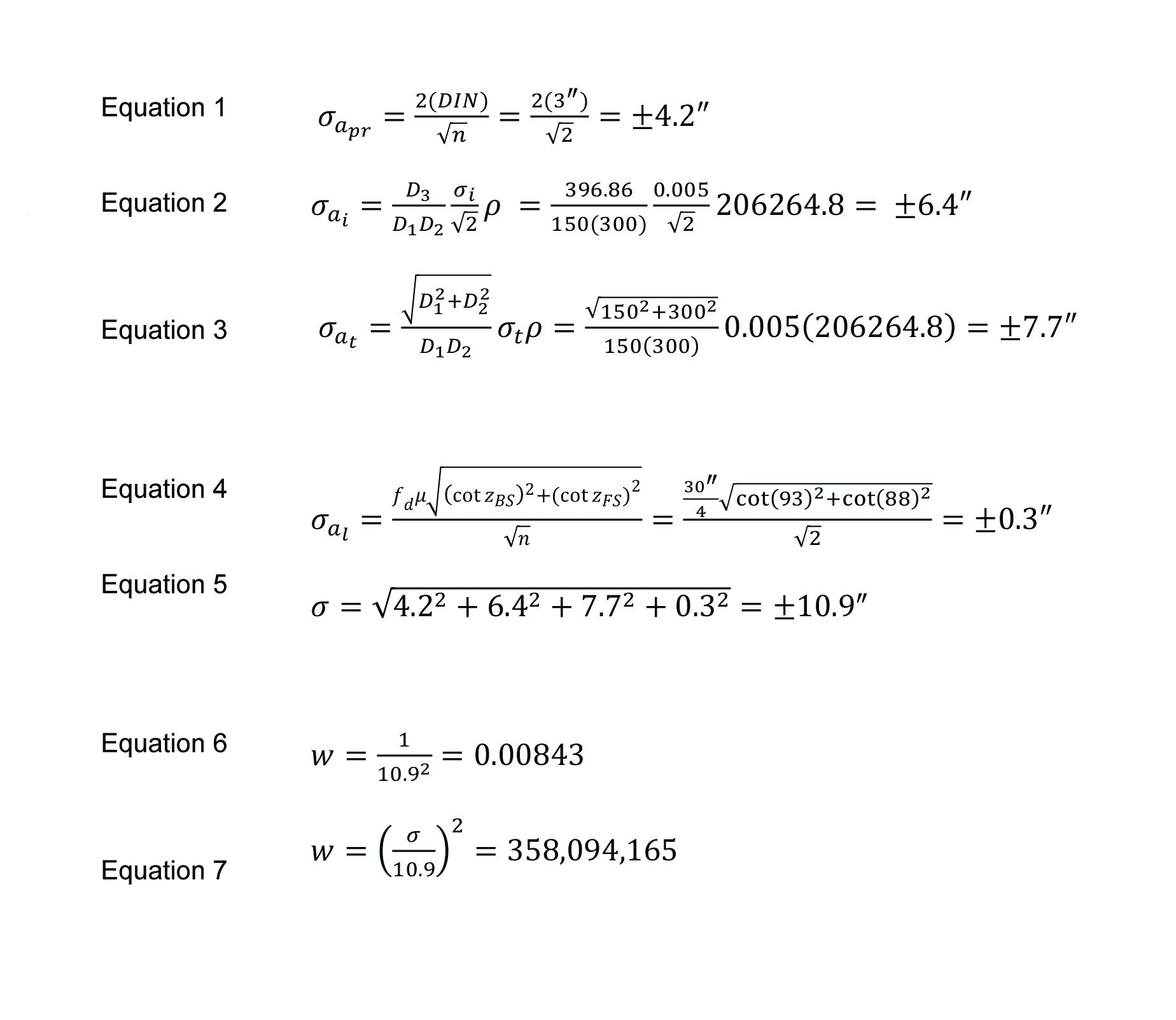
Suppose an angle of size 120° is observed with a total station having an ISO specification of 3”. It is observed 1DR with a backsight distance of 150 ft and a foresight distance of 300 ft. The zenith angle to the foresight was 93° and to the backsight was 88°. The angle was observed 1DR (n = 2). The 30” level bubble was kept to within ¼ of a division.
What is the estimated uncertainty in the angle if the setup errors were assumed to be within ±0.005 ft? What is the estimated weight of the observation? (Refer to Part 3 in this series of articles for the definitions of the variables.)
Solution
Error due to pointing and reading: as in Equation (1).
Error due to instrument miscentering: as in Equation (2).
Error due to target miscentering: as in Equation (3).
Error due to instrument misleveling: as in Equation (4).
Note that the instrument leveling error is insignificant for most surveys, typically, and thus is ignored, typically. It only needs to be considered when the vertical angles become large.
Estimated standard error for the angle is: as in Equation (5).
The weight for this particular angle observation is in Equation (6) in units of seconds or as in Equation (7) in radian units.
If you wish to achieve a “correctly weighted least squares adjustment,” you can see from the above and previous articles that, estimating an appropriate weight for your observations is not an easy task. Is this important? Most definitely, and this goes beyond the ALTA/NSPS standards.
How This Came to My Attention
I started down this road in the early 1980s. As a graduate student I wrote much of the software used by other graduate students in their research. In my software was an option to use statistical blunder detection to find blunders in the data (a future article).
A friend who was a licensed land surveyor in Wisconsin had encountered a problem in his research project. As was the norm back then, he brought this problem to me. It was noted that the linear misclosure of a traverse that bounded two and one-half public land sections was 10 ft! The theodolite used at the time had a 1-min least count, for which he estimated that he could read the angles to the nearest 0.3’ of a minute.
He had given every angle, regardless of the length of the sight lines or its size, an estimated uncertainty of ±18” in the software, but the software’s post-adjustment blunder detection could not isolate the observation with the blunder even though he had numerous observational checks/redundant observations.
On one particular station he had observed multiple angles over several different days in varying combinations. I implemented the weighting scheme by estimating the standard errors for each observation, and the statistical blunder detection identified one angle on the opposite side of the closing course.
Although my memory is getting long in the tooth (30+ years!), I believe it differed by only 6”″ (0.1’′) from the other angles at that station that had been observed in varying combinations. It had extremely short sight distances compared to the other angles in the traverse. Obviously, its error was more than 18” but that is what the weighting model had given it for a precision.
More important is that many of the other angles with long sight distances also had an estimated error of ±18”. I couldn’t believe it any more than he nor you probably can, but that one angle, which had an error less than the least-count of the instrument, had opened the traverse by 10 ft at its closing point. The proof was when the angle was removed, the traverse closed extremely well, which is a testament to his measuring abilities.
A few years later, this happened a second time in a network that covered a 50-ac parcel of land where the angular error was caused by students when the target occupied a different point on the section corner monument than occupied by the instrument. The sight distances on these angles were only about 100 ft in length. Again, the angular error was well below the reading capabilities of the instrument.
The software identified the observation, but when the students repeated the observations they repeated the same jobs, and thus the same problem occurred. It wasn’t until they discussed their field procedures that they realized that they had occupied two different points on the cap. Now, why it had two points I leave to the surveyor who set the section corner monument to explain!
These incidents demonstrated to me the need to get the weights on the observations correct, and the power of statistical blunder detection.
Since then I have repeatedly used this technique in all my adjustments, which was rather easy since I implemented this handful of equations from the previous articles in this series into my software. Unless there is a blunder in the data, I never fail to pass the “goodness of fit/x2 test.” I also never use the sample standard deviations to determine the weights.
Additionally, since I have estimated the standard errors for each observation, I often use the critical value from the t distribution and the estimated standard error for the observation to isolate blunders in data. I discuss this technique in an earlier article but will repeat it here.
Try It Yourself
To see how this is done, assume that the estimated standard error in an angle using the previously described equations is ±2.7”. Further, assume that, after the least squares adjustment with 15 degrees of freedom (redundant observations), I have a residual for this angle of −10.8”. The critical t value for this adjustment at 0.003 level of significance is t0.0015,15 = 3.54. Multiplying 3.54 and 2.7”, I find that an acceptable range for the residual of this observation is ±9.6”. Since the residual of −10.8” is outside of this range, I have a 99.7% probability that this observation is a blunder.
When I am working on example problems for my book on adjustment computations, I often insert intentional blunders in the data. The reason I do this is to allow instructors to teach not only the mathematics of least squares but more importantly the proper techniques used to build a valid stochastic (weight) model and analyze the data after the adjustment is performed.
By the way, the instructor’s manual that accompanies the book informs the instructor of the magnitude of the blunder and the observation. Note that this manual is available only to instructors. In doing this, I can’t recall a single instance where the critical value from the t distribution times the observation’s estimated standard error did not identify the blunder that was inserted. This is true even in a few instances where post-adjustment statistical blunder techniques failed.
But, here is the unfortunate part. Although these techniques have been written about by R. Ben Buckner, Ed Mikhail, Gordon Gracie, and myself, I know of no commercial software package that implements this method of estimating standard errors before a least squares adjustment. Most software allows you to put in setup errors, but they then default to sample standard deviations with default values to handle the situation when the standard deviation of an observation is zero.
How to Implement This Method
There are only two options if you wish to implement this method of estimating standard errors for your observations. One is to write your own software. I had my students do this by creating an Excel spreadsheet in their third semester. For those wishing to do this, my book entitled Adjustment Computations provides the development of the equations in Chapter 7.
The other approach is to start requesting that manufacturers produce software that implements this method of estimating the standard errors for your observations.
You don’t think this will ever happen? I was giving a least squares workshop in Corvallis, Oregon, several years ago, and several of the TDS programmers were in my class. At one point I asked the programmers why their software contained an option that had no theoretical background to it. The response was because the surveyors had asked for it.
So, don’t be afraid to ask. One request may fall on deaf ears, but hundreds of requests will not. After all, they are in the business to sell to you, and you need to create a “correctly weighted least squares adjustment” to satisfy the ALTA/NSPS land title surveys as well as to properly identify blunders in your data.
You have the need, and they can easily implement these equations in their software where all you need to provide is the number of times you turned the angle, estimate the set up errors, and
enter the manufacturer’s specifications for the instruments used in the survey.
Hopefully, you now realize that the sample standard deviation computed from two repetitions of an angle is not statistically reliable enough for weighting your adjustment. The only method to get a “correctly weighted least squares adjustment” is to compute it based on the theory of error propagation in measurements.
I will return to the topic of blunder detection after discussing the last of the sampling distributions important to surveying, which is the F (Fisher) distribution. Until then, happy surveying.
References
ALTA/NSPS. 2016. “Measurement Details for 2016 ALTA/NSPS Land Title Surveys” accessed at https://nsps.site-ym.com/?page=ALTAACSMStandards on Mar 31, 2016.
Buckner, R.B. 1983. Surveying Measurements and Their Analysis. Landmark Enterprises, Rancho Cordova, CA.
Ghilani, C. 2010. Adjustment Computations: Spatial Data Analysis. Wiley & Sons, Inc., Hoboken, NJ.
Mikhail, E. and G. Gracie. 1981. Analysis and Adjustment of Surveying Measurements. Van Nostrand Reinhold, New York, NY.